Plotting
x<-1:10
y<-21:30
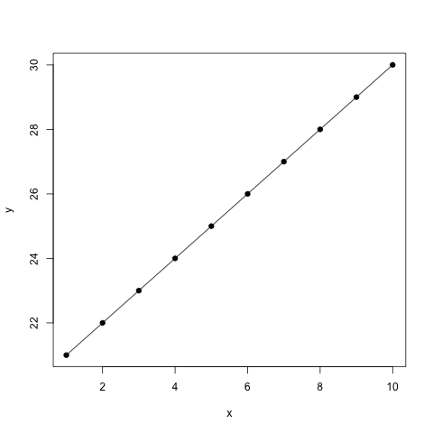
plot(x,y) // simplest plot
plot(x,y,type="o") // different types: p(oints), l(ines), b(oth), c, o(verplotted), h(istogram like), n(one)
plot(x,y,type="o",pch=19,lty=1,lwd=1) // point character 19, line type 1 and line width 1
plot(0:25,pch=0:25) // most of the predefined point characters
plot(x,y,type="o",pch="M") // but loads of other characters are possible
lty(1:6)
lwd(1:7)
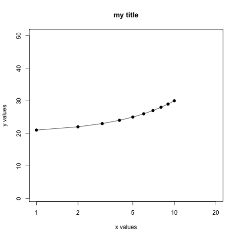
plot(x,y,type="o",pch=19,lty=1,xlim=range(1:20),ylim=range(1:50),xlab="x values",ylab="y values",main="my title",log="x")
// ranges and labels on axes, title and semi-log scale
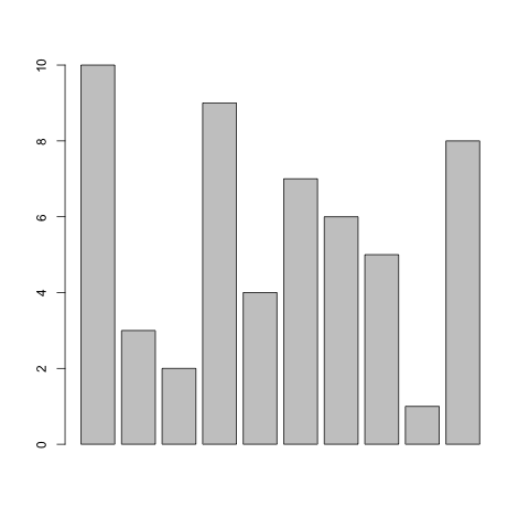
x<-sample(1:10)
barplot(x) 				// simple barplot
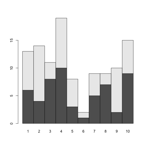
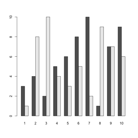
y<-sample(1:10)
xy<-rbind(x,y)
barplot(xy,space=0,names.arg=1:10) 	// matrix, stacked bars, w/o gap between bars, bar labels
barplot(xy,names.arg=1:10,beside=T) // same but next to each other, space != 0
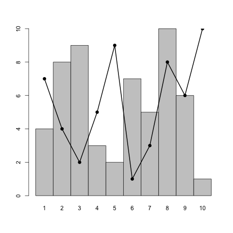
mybar<-barplot(x,names.arg=1:10) 	// create variable for plot
lines(mybar,y,type="o",pch=19,lwd=2)	// add line which points according to x-axis
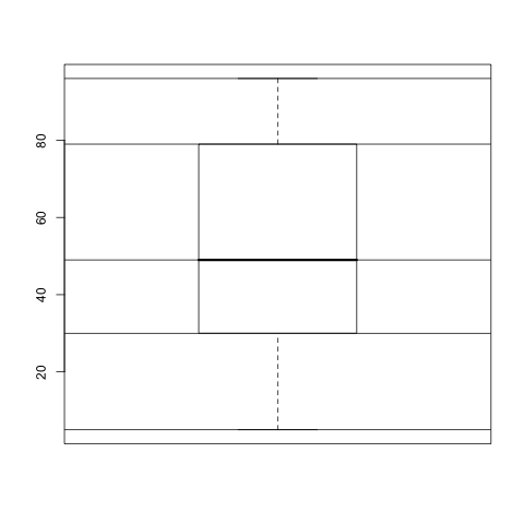
x<-sample(1:100,30,replace=T)		// sample vector
boxplot(x)				// box-and-whisker plot

abline(h=median(x))			// median (second quantile) of vector
abline(h=min(x))			// min value of vector
abline(h=max(x))			// max value
abline(h=quantile(x,type=2)[[2]][1])	// first (lower) quantile (cut off first 25%)
abline(h=quantile(x,type=2)[[4]][1])	// third (upper) quantile (cut off first 75%)
x1-sample(1:100,30,replace=T)
x2<-rnorm(50)
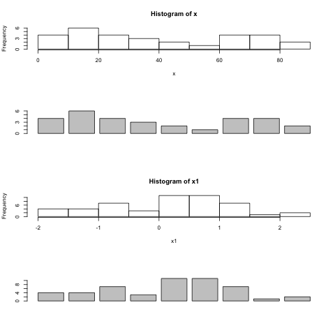
par(mfrow=c(4,1)) // one way to split the canvas: mfrow=c(rows,cols)
myhist1<-hist(x1) // histogram
barplot(myhist1$count) // same result with barplot
myhist2<-hist(x2) // more typical looking histogram
barplot(myhist2$count) // again same with barplot
Misc Plotting Functions [source]
Points, Lines, Colors
points() lines() // add points and lines to existing plot
abline(a=5,b=0.3,h=0,v=0) // draw straight line a=y-intercept, b=slope, h=y-value for horizontal,
// v=x-value for vertical line
segments(2,7,9,1,lty=2,lwd=4,col="red") // plot a segment from [x1,y1] to [x2,y2]
colors() // returns all colors
colors()[grep("red",colors())] // returns all colors containing "red"
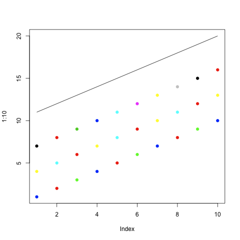
mycols<-c("blue","red","green")
mycols1<-c(rgb(255, 255, 0, maxColorValue=255),rgb(0, 255, 255, maxColorValue=255),rgb(255, 0, 0, maxColorValue=255))
plot(1:10,ylim=range(1:20),pch=19,col=mycols) // 10 points with repeating color
points(4:14,pch=19,col=mycols1) // 10 points from different color vector
points(7:17,pch=19,col=1:10) // predefined colors
lines(11:20) // just a line
 picture taken from: http://www.mzandee.net/~zandee/statistiek/R/Rlecturenotes.pdf
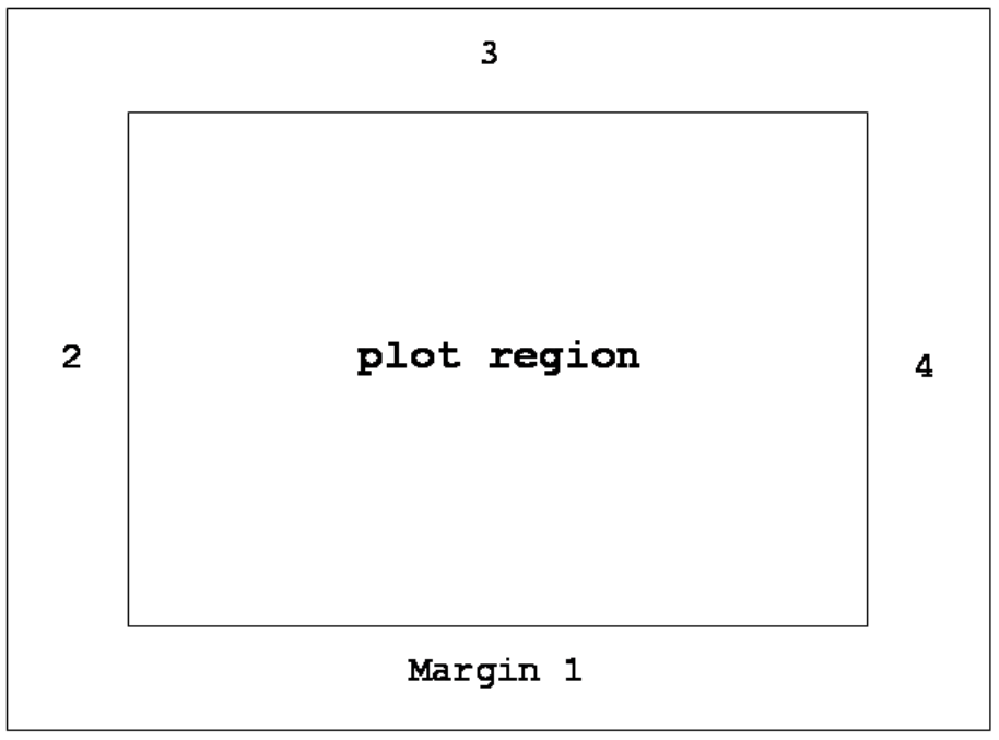
mtext("hello plot 1",1) 	// print text at one of the 4 sides, 1=bottom
mtext("hello plot 2",2) 	// 2=left
mtext("hello plot 3",3,cex=5) 	// 3=top, large font
mtext("hello plot 4",4) 	// 4=right
Axes
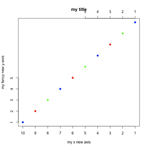
plot(1:10,pch=19,col=mycols,ann=F,axes=F)	// plot w/o annotations and axes
axis(1,at=1:10,labels=10:1,cex=0.5)		// add bottom x-axis w/ reverse labels
axis(2,at=1:5)					// add left y-axis but only from 1..5
axis(3,at=6:10,labels=5:1)			// add second x-axis
box()						// draw box around plot
title(main="my title",xlab="my x new axis",ylab="my fancy new y-axis")
						// add title, xlab and ylab
Legend
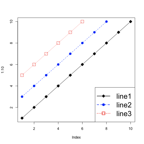
plot(1:10,type="o",pch=18,lty=1,cex=2,col="black") 	// black line1
lines(3:10,type="o",pch=20,lty=2,cex=2,col="blue")	// blue line2
lines(5:10,type="o",pch=22,lty=3,cex=2,col="red")	// red line3
legend("bottomright",c("line1","line2","line3"),pch=c(18,20,22),lty=1:3,col=c("black","blue","red"),cex=2,lwd=2)
							// legend w/ all parameters used in the plot
						// re-define plotting area
par(fig=c(0,1,0.5,1),mar=c(5,5,2,3))
						// coordinates of the figure region: fig=c(x1,x2,y1,y2)
						// margin to borders: mar=c(bottom, left, top, right)
plot(1:10)
par(fig=c(0,1,0,0.5),mar=c(5,5,2,3), new=TRUE)	// re-define where to plot
plot(sin(1:10),type="l")
par(mar=c(5,4,4,2)+0.1)				// reset to defaults
Output to a file
png(filename="myfile.png", height=768, width=1024, bg="white")
pdf(file="myfile.pdf", height=7, width=13)
postscript(file="myfile.eps",onefile=FALSE,horizontal=FALSE,height=7,width=7,pointsize=14)
dev.off()		// close device