This document describes our next step after the CDX based profiling. The document has two major sections. The first section talks about the trend of precision, recall, and specificity of various profiling policies as we incrementally learn more about the archive holdings via sampling. The section concludes that a smaller (less detailed) profiling policy is suitable when a very small fraction of the archive holdings is known, otherwise, a more detailed profiling policy is a better choice. The second section talks about the fulltext search based profiling. It describes the Random Searcher Model that operates in various modes to perform the search and discovery, measures their cost and learning rate, and concludes the best performing search and discovery mode.
So far in our CDX analysis we were assuming that the profiler has access to the complete CDX data. As a result all profiling policies resulted in 100% recall hence no false negatives. Consequently, the effort was made to minimize the number of false positives. We found that a higher order profiling policy (one with more details) yields better results, but costs more. We ran our experiments on 23 different profiling polices and found that we can group some policies together that perform almost similar then we can pick one from each group for further analysis. Here are our picks:
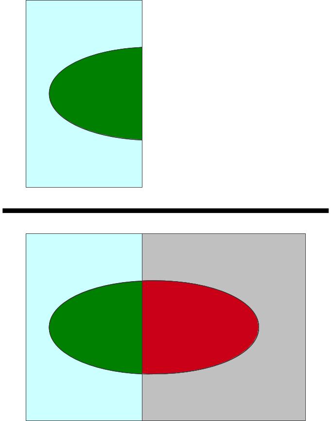
We now move to sampling based profiling where we do not profile the complete archive, instead a fraction of it is known. Then we predict the presence of a URI in the archive based on our partial knowledge. This approach will yield some false negatives as well. Hence, it is important to analyze the confusion matrix (false positives, true positives, false negatives, and true negatives) of each profiling policy as a function of the fraction of the archive known.
To make the confusion matrix, we first take a sample URI set.
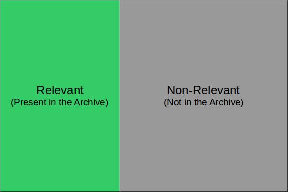
Then we select and archive and for each URI from the sample set we check the archive to see if the URI is present in that archive. This divides the sample URI set in relevant and non-relevant subsets.
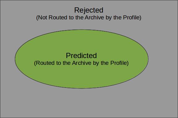
We then select a profiling policy to build a (complete or partial) profile of the selected archive. Using this profile we check each URI from the sample set whether it is routed to the archive. This routing prediction based on the profile divides the sample set in two subsets (roted and not routed).
The superimposition of the above described subsets divides the sample set into four subsets false positives (FP), true positives (TP), false negatives (FN), and true negatives (TN) as illustrated in the figure bellow.
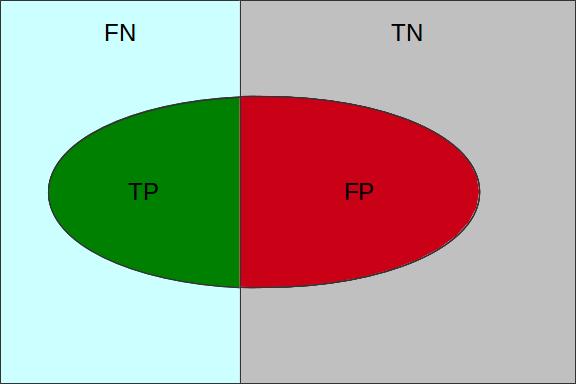
| Present in the Archive | Not in the Archive | |
|---|---|---|
| Routed to the Archive | True Positives (TP) | False Positives (FP) |
| Not Routed to the Archive | False Negatives (FN) | True Negatives (TN) |
For this analysis we selected the early ten years of UKWA dataset as the gold dataset. Then we extracted the unique URI-Rs from it and randomized it. The randomized URI-R list was then split into ten equal chunks. We then profiled these chunks incrementally using different policies to see how these policies perform when we know only 10%, 20%, 30%... to 100% of the archive. In each case we calculated the confusion matrix. Later we plotted Precision-Recall and Specificity-Recall on these increments to analyze the trend.
In the information retrieval terms, four sample sets (that we created earlier), each containing one million unique URI-Rs will act as four different corpuses, profiling policies will act like search keywords, various incremental profiles will work like indexes, and relevance judgment will be done based on the overlap of the sample URI sets and the ten years of UKWA URIs.
How often relevant items are found in the sample? [(TP+FN)/(TP+FN+TN+FP)] -- In Memento routing terms, how many of the sample URIs are actually present in the archive. A low Prevalence value indicates that the sample is sparsely archived. Therefore, the Precision value may not be significant.
How often relevant items are selected? [TP/(TP+FN)] -- In Memento routing terms, how often lookups were routed by a profile to an archive that holds them out of all the lookups that were present in that archive. Recall is very important, because it determines how many relevant items can we afford to let go to compromise with other factors such as cost.
How often selected items are relevant? [TP/(TP+FP)] -- In Memento routing terms, how often lookups routed by a profile to an archive are actually held by that archive out of all the routed lookups. Precision gives a sense of how much false positives each policy brings as we increase the recall. However, it does not tell anything about the true negatives that were successfully discarded.
How often non-relevant items are discarded? [TN/(TN+FP)] -- In Memento routing terms, how often lookups were not routed by a profile to an archive that actually did not hold them out of all the lookups that were not present in that archive. In other words, Specificity is to the negative class what Recall is to the positive class. Specificity is very important in routing analysis because it reflects the ability of the router to correctly identify the non-relevant items and discard them. This becomes even more important when the Prevalence is low. In our study we found that less than 5% of the queried URIs have mementos in any individual archive that is not the Internet Archive. Hence, the precision is often skewed.
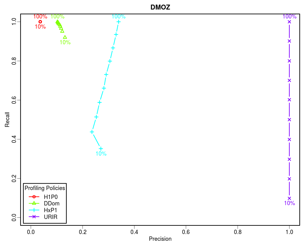
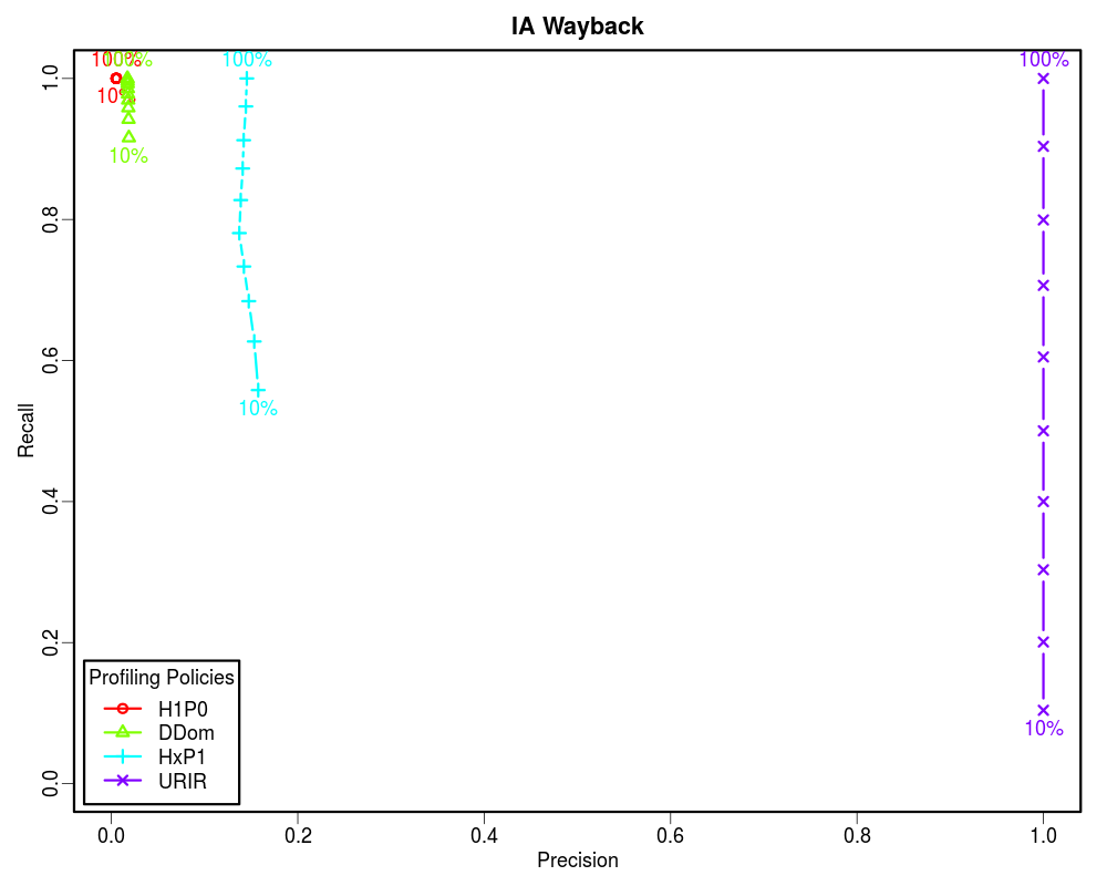
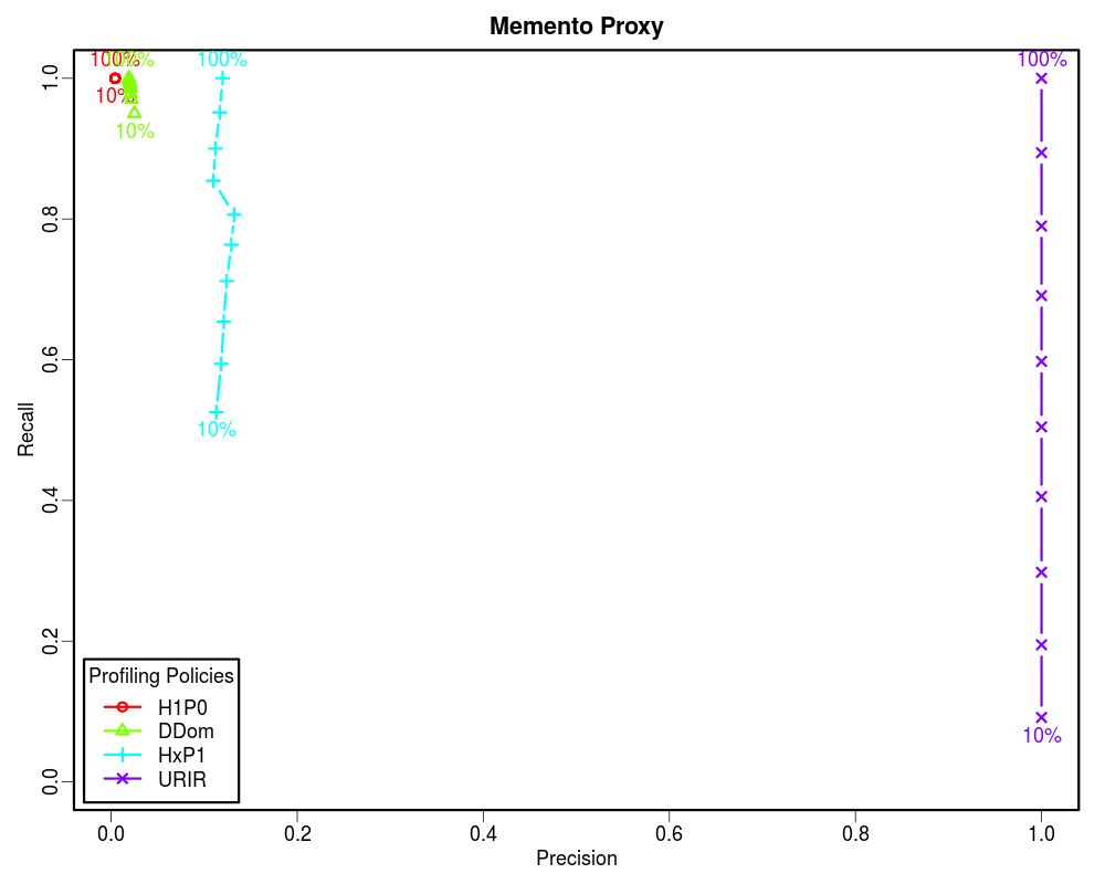
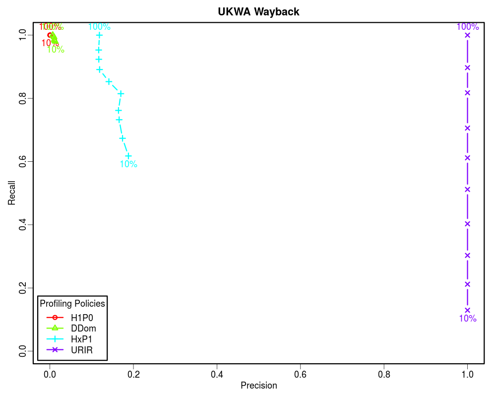
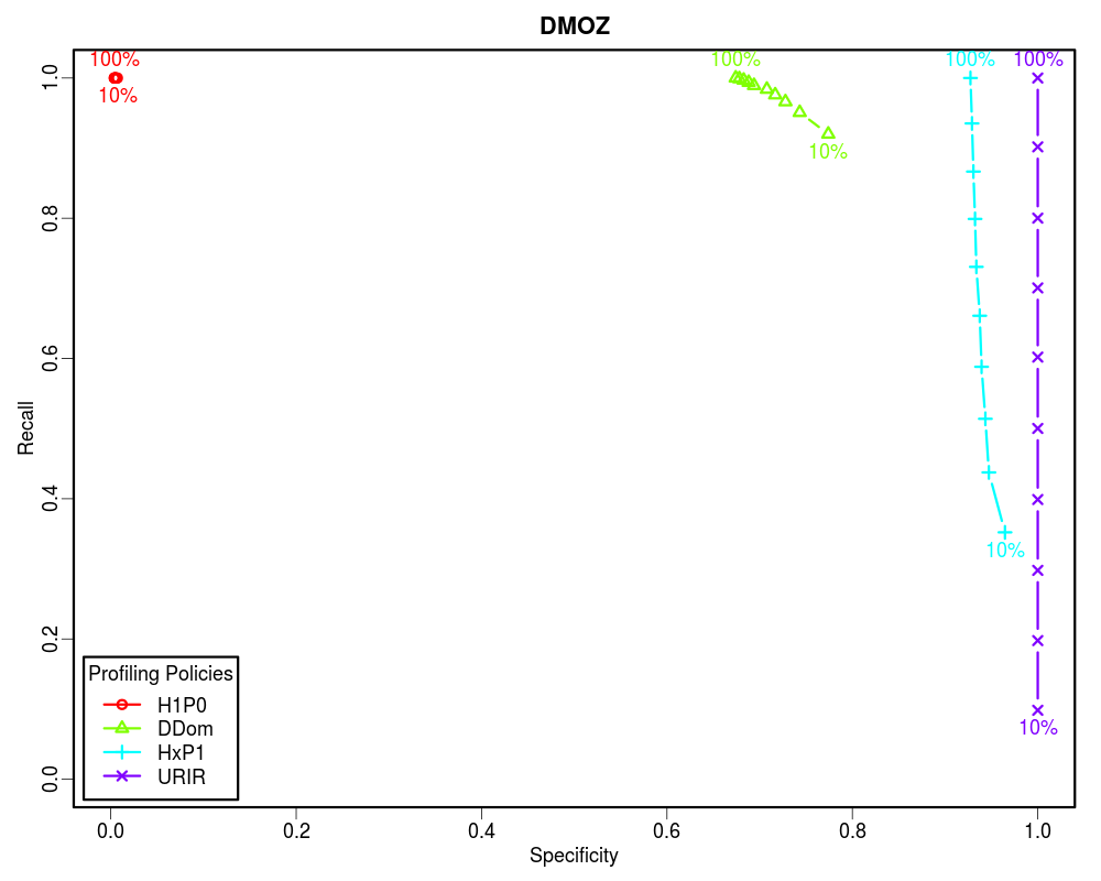
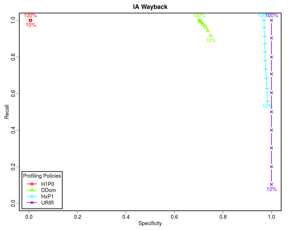
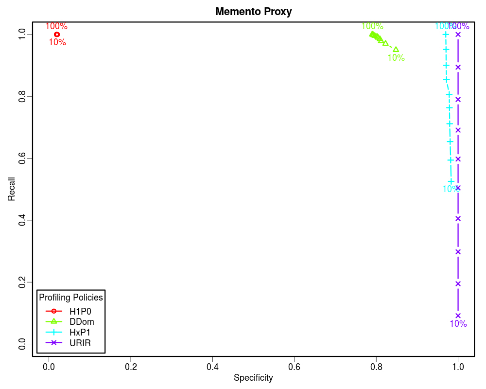
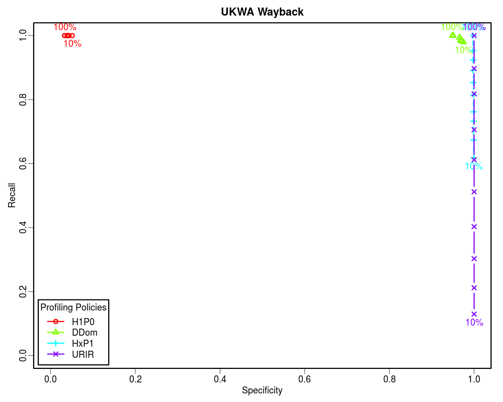
Since the Prevalence of our samples is less than 0.05, the Precision vs Recall graphs are not good indicators of the routing efficiency. However, the Specificity vs Recall graphs can be used to estimate the routing efficiency of different profiling policies as a function of how much of the archive holdings we know. From these graphs it is clear that if the complete archive is known, we should choose higher order profiles such as HxP1. The HxP1 profile has the Specificity (the ability to not route non-relevant URIs to the archive) almost as good as the URIR profile. From our earlier work we know that the cost of the HxP1 profile is less than one sixth of the cost of the URIR profile. Additionally, the HxP1 profile has higher Recall than the URIR profile when the complete archive is not known. However, since we cannot afford to lose so much of the recall, we should go for smaller profiles such as DDom when we have partial access to the archive (such as when using fulltext search). Above graphs show that a DDom profile (that has less than 1% cost as compared to the URIR profile) can have about 0.9 Recall while successfully rejecting about 80% of the non-relevant URIs by only knowing 10% of the archive. Cases where only a tiny fraction of the archive is known by sampling (such as when neither CDX is available nor fulltext search), we should go for the smallest profile H1P0/TLD-only to maintain an acceptable Recall value. The URIR profile, though always yields 100% Precision and Specificity, it suffers from the poor Recall. Even if the complete CDX is accessible, the URIR policy costs a lot as compared to other policies. Additionally, the URIR policy does not have any predictive powers for unseen URIs, hence maintaining the freshness of the profile is challenging as the archives collect more stuff.
Gaining access to the CDX files of many archives is a challenging (and often impossible) task, but keeping them up-to-date is even harder. Fulltext search is another way to know about the holdings of an archive. In this approach, we send some random query terms to the archive and collect the resulting URIs returned from the archive. Although with each successful response we learn some new URIs, but this learning rate slows down as we go forward because of the fact that some of the URIs returned in a response may have been already seen in earlier attempts. This follows the Heaps' Law.
With carefully chosen values of various advanced search attributes and selection of suitable list of keywords we can affect the parameters of the Heaps' Law and maximize the learning rate. In this section we analyze different fulltext approaches to discover holdings of an archive. We also explored different ways to perform the search when the language of the archive is unknown or a list of suitable keywords is not available for that language.
For our experiments we chose Archive-It hosted North Carolina State Government Web Site Archive collection which is the largest collection on the Archive-It and provides fulltext search feature. Since we have Archive-It data (up till 2013) hosted in our dark archive at ODU, it was easier for us to perform the coverage analysis on this dataset.
We started our experiment by searching for stop-words. For example when we searched for the term "a" it returned 26M+ results that is very close to the number of the HTML resources in the collection until March 2013. However, each page only contains 20 results, hence, in order to learn all the 26M+ URIs, we will have to make 1.3M+ HTTP GET requests. Our goal was to make as few requests as possible to learn enough diverse set of URIs in the collection. Additionally, this approach cannot be generalized as not all archives will behave the same on stop-words.
In the next step we decided to build static or dynamic word lists and search for those words as query terms. For each term we only record the URIs in the first resulting page and move on to the next word in the list. Having a configurable result pagination would have benefited us by setting up a larger number for per page results, but Archive-It has it fixed to 20 and does not allow changing that.
We collected top 2,000 English nouns and used them as the query terms against the collection. We accumulated the first page results to plot the learning curve, but also extracted other information such as the result count for each search term. As expected, these top terms yielded high values for the result count for each terms. Additionally, each term yielded more than one page of result, hence no effort was unsuccessful. We also observed that the response time is correlated with the result count, so same number of top terms would take longer total time than a random word list.
We ran same procedure on randomly chosen 2,000 unique words from the built-in Linux dictionary. This time the average number of results per terms was lower, but there were many terms for which the collection returned no results or less than 20 (page size) results.
The above two experiments were based on the static lists of words. This static word list approach requires the knowledge of the language (and field) of the collection to choose a static list of words for that language which may not be easily available. Additionally, the list would be finite and may not be enough to discover enough of the collection holdings. To overcome this issue, we build a model to dynamically discover new words from the searched pages and utilize those words to perform further searching. We introduced three different variations of the dynamic discovery model based on how the new words are learned and how the next word for searching is chosen. We then analyzed the learning rate and HTTP cost of each variation.
In this section we elaborate on different searching approaches algorithmically that we utilized in the previous section. We develop a general Random Searcher Model that can be configured to operate in one of the four modes with the help of different configurable policies.
The Random Searcher Model has following data structures:
The Random Searcher Model has following policy configurations:
Not all possible policy permutations are valid. Following tree (with the hierarchy "Vocabulary Seeding Policy" > "Word Selection Policy") illustrates four valid policy configurations that yield in four different operation modes of the Random Searcher Model.
The table below maps Random Searcher Model operation modes with corresponding sets of policy configurations. Operation modes are named after the corresponding uniquely identifying policy values.
| Random Searcher Model Operation Mode | Vocabulary Seeding Policy | Word Selection Policy |
|---|---|---|
| Static | Static | Select All |
| Popularity Biased | Progressive | Popularity Biased |
| Equal Opportunity | Progressive | Equal Opportunity |
| Conservative | Conservative | Select All |
The Random Searcher Model has following public procedures (it may have additional internal utility or abstraction methods in the implementation):
To run the Random Searcher an instance of the Random Searcher Model is initialized with one of the four possible modes, some initial seed words, termination condition configuration, tokenizer pattern, and other configurations. The the NextWord generator is iterated over to discover next word for searching until it hits the termination condition. For every word the search method is called which internally performs the collection lookup and updates various data structures of the Random Searcher instance. Once the iterator terminates, GenerateProfile method is called to serialize collected statistics in an Archive Profile. Please see the appendix section for pseudocode of these methods.
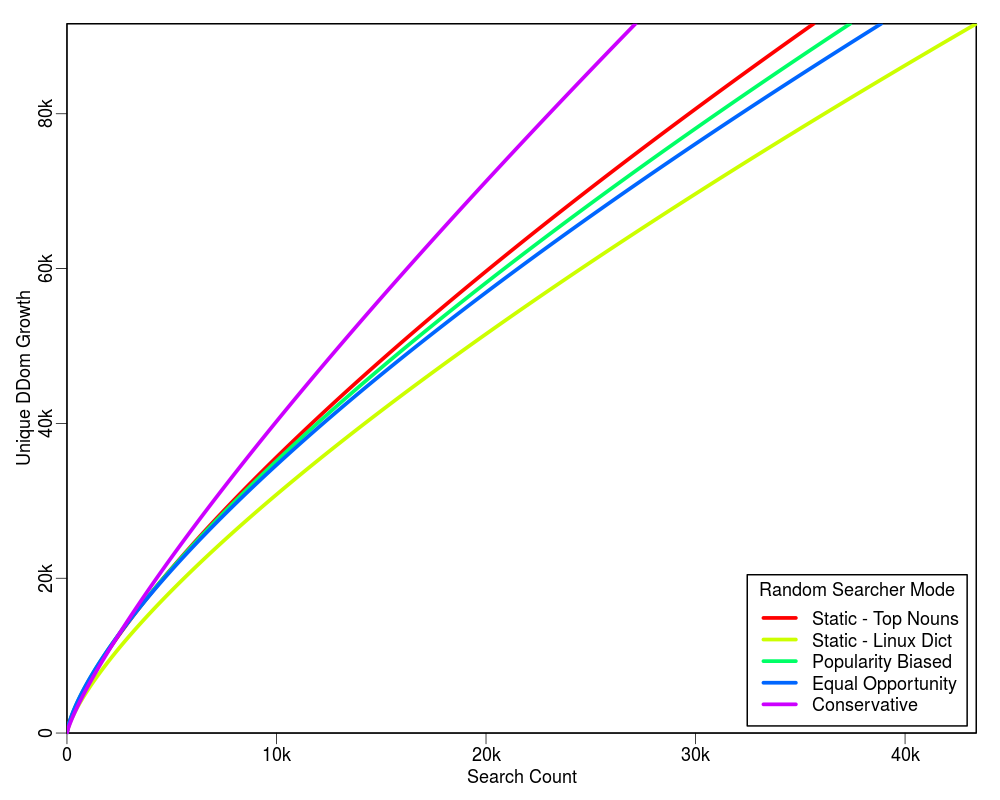
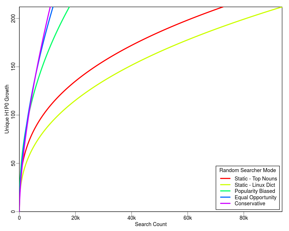
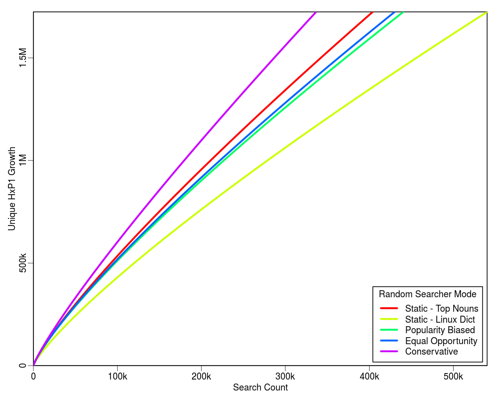
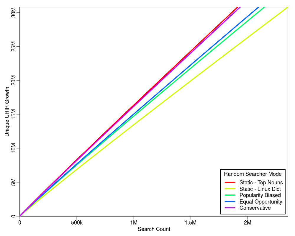
Following graphs show the projected estimate of the search cost for each of the four profiling policies based on the initial 2,000 searches. Each graph is extended up to the 100% limit of each profiling policy on the Y-axis. For example, there are total 212 unique TLDs in the collection, hence the upper Y-axis limit in the first plot is set to 212.
The table below shows the HTTP cost of each mode with respect to the corresponding query cost. The value of "delta" is quite small as compared to "C". In our experiments we found that for C = 2,000 the value of delta was 8.
| Operation Mode | Query Cost | HTTP Cost |
|---|---|---|
| Static | C | C |
| Popularity Biased | C | 2 * C |
| Equal Opportunity | C | 2 * C |
| Conservative | C | C + delta |
From the above plots we conclude that the "Conservative" mode is an overall winner. It shows a higher learning rate and does not require a static list of words to be supplied. It is also good because it does not have much overhead HTTP request cost for the term discovery.
do# Initialize policiescase config.modewhen "Static"VocabularySeedingPolicy = "Static"WordSelectionPolicy = "Select All"when "Popularity Biased"VocabularySeedingPolicy = "Progressive"WordSelectionPolicy = "Popularity Biased"when "Equal Opportunity"VocabularySeedingPolicy = "Progressive"WordSelectionPolicy = "Equal Opportunity"when "Conservative"VocabularySeedingPolicy = "Conservative"WordSelectionPolicy = "Select All"elseprint "Unknown operation mode: "# Initialize VocabularyVocabulary = config.seed# Initialize other factors such as termination condition and tokenizer patternend
do# Returns True or False based on various factors such as:# - Vocabulary Seeding Policy# - Sates of Vocabulary, SearchLog, or ResultBank# - Average learning rate of last K searches# - Time spent etc.end
do# Unless termination condition is met# If Vocabulary is empty# Return a randomly selected successful searched word from the SearchLog# Else# Return a randomly popped word from the Vocabulary# Return nilunless TerminationCondition()if Vocabulary.empty?return SearchLog.select_random_successful_searched_word()elsereturn Vocabulary.pop_random_word()endendreturn nilend
do# Search for the word# Unless search result is empty# Update SearchLog# Update ResultBank# Unless Vocabulary Seeding Policy is "Static"# Unless Word Selection Policy is "Select All" and Vocabulary is not empty# Select a random URI from the result# Extract words from that URI# If more than one unique extracted words# Overwrite Vocabulary with the extracted wordsresponse = Collection.search(word)results = response.resultsunless results.empty?SearchLog.add(response)results.each do |res|ResultBank[res.urir] = res.urim_countendunless VocabularySeedingPolicy == "Static"unless WordSelectionPolicy == "Select All" && Vocabulary.empty?uri = results.random().urimwords = ExtractWords(uri)if words.unique_count > 1Vocabulary = wordsendendendendend
do# Fetch the page at the given URI# If content found in the success response# Strip markup, styles, and scripts# Extract tokens using tokenizer pattern# Clean any invalid or empty tokens# Unless Word Selection Policy is "Popularity Biased"# Remove duplicates# Return unsorted list of tokenswords = []response = http.get(uri)if response.successtext = response.body.strip(markup, styles, scripts)tokens = text.split(tokenizer_pattern)words = tokens.filter_invalid()if WordSelectionPolicy != "Popularity Biased"words = words.unique()endendreturn wordsend
do# Initialize a profiler with a given profiling policy# Initialize a profile with the meta information# Iterate over the ResultBank and generate profiling keys from each record# Add URI Key with corresponding URI-M count in profile stats# Serialize the profileprofiler = Profiler(policy)profile = Profile(config)stats = {}ResultBank.each do |urir, urim_count|key = profiler.generate_key(urir)stats[key] += urim_countendprofile.apply(stats)selrialize(profile)end
do# Initialize a Random Searcher with desired mode, seed words, and other configurations# Iterate over the NextWord generator until the termination condition is met# Call search method of the Random Searcher on the current word# Generate profilers = Initialize(config_object)while word = rs.NextWord()rs.Search(word)endrs.GenerateProfile(profiling_policy)end