


Choosing Tests
Steven Zeil
Abstract
Testing starts with the design of test cases that express our strategy for testing our code. Where do these come from?
Testing strategies are generally divided into three categories:
-
Blackbox testing chooses tests based upon the requirements, without consulting the implementation. In fact, black-box tests are often developed before coding has even begun.
-
Whitebox testing chooses tests based upon the details and structure of the implementation.
-
Representative testing chooses test data based upon projections of how the program will be used in operation.
We will examine each of these possibilities.
1 Types of testing
We can differentiate testing strategies by overall goal:
-
Statistical testing
- tests designed to reflect the frequence of user inputs.
- Used for reliability estimation.
-
Defect testing
- tests designed to discover system defects.
- A successful defect test is one which reveals the presence of defects in a system.
Choosing Test Data
From these motives come different approaches to choosing test data
-
Representative testing
- tests designed to reflect the frequence of user inputs.
- Used for reliability estimation.
-
Directed testing
- Tests designed to discover system defects.
- A successful directed test is one which reveals the presence of defects in a system.
2 Representative Testing
Choose data that is representative of the way the end users will exercise the software.
- Advantages:
- realism — catches the kinds of failures that the users would have encountered
- relatively cheap to generate tests
- time to failure during test reflects time to failure in operation
- useful in statistical reliability modeling
Producing Representative Tests
Test data can be obtained via
-
collected data from an existing system
A useful option when we are modifying an existing system, which is probably more common than projects where we build a new system from scratch.
“System” here is generic. Even if the old system was completely manual, we may be able to collect and then digitize input data to the old system.
-
further selection may be needed
-
cannot accomodate new functionality
-
-
random generators
-
non-uniform, to match desired distribution
The conventional
rand()function yields a uniform distribution — each possible output is equally likely. But random number generators can be implemented for just about any probability distribution – normal, exponential, etc. -
can be hard to generate non-numeric ADT values
Think about the problem of generating random
strings to serve as names. If you simply generate sequences of randomly selected length containing randomly selected characters, the results won’t be very name-like and may strain the ability of code for dealing with fist & last names, etc. Such random strings also tend to look alike ot the human eye, making the visual evaluation of test output nearly impossible.What I have done in the past is to get lists of common first names and separate lists of real last names (publicly available U.S. census data is great for that, BTW). Then randomly select one first name and one last name and combine them together. Granted, you do get some interesting ethnic combinations that way, e.g., “Nguyen Smith” or “Antonio O’Reilly”.
Now consider the further problem of randomly generating a list of customer transactions, of which these names are one component. Now you have the further problem of how often a particular customer name should be repeated. If you randomly generate a name for each transaction, you will wind up with almost no repeats, and that could lead to some very unrealistic transaction sequences.
-
Representative Testing
- Requires an operational profile for its definition
- The operational profile defines the expected pattern of software usage
2.1 The Operational Profile
The operational profile is a description of the probability distribution of the input.
It describes how often, during operational program use, certain “kinds” of inputs will be seen.
Sample Op Profile
| Input Category | Percentage | |
|---|---|---|
| Transaction Proc. | 85% | |
| Balancing | 14% | |
| Year-end Report | 1% | |
For an accounting program, we might start with an observation that past activities have broken down like this.
- But then we might note that transactions come in many different kinds…
Sample Op Profile
| Input Category | Percentage | |
|---|---|---|
| Transaction Proc. | 85% | |
| New account | 7% | |
| Close account | 3% | |
| Debits | 70% | |
| Credits | 20% | |
| Balancing | 14% | |
| Year-end Report | 1% | |
- After noting that the requirements specify different behaviors for transaction on existing accounts and non-existent accounts, we might look at company records for still more statistics…
Sample Op Profile
| Input Category | Percentage | ||
|---|---|---|---|
| Transaction Proc. | 85% | ||
| New account | 7% | ||
| new | 90% | ||
| already exists | 10% | ||
| Close account | 3% | ||
| non-existent | 15% | ||
| exists | 85% | ||
| Debits | 70% | ||
| non-existent | 25% | ||
| exists | 75% | ||
| Credits | 20% | ||
| non-existent | 25% | ||
| exists | 75% | ||
| Balancing | 14% | ||
| Year-end Report | 1% | ||
The breakdown of transactions into cases bases on whether the account is new (non-existent) versus already existing suggests something of an answer to the earlier discussion of randomly generating customer names and asking how often they should repeat. By explicitly measuring how often a new transaction involves an existing account, we know whether to randomly generate a new name or to randomly select from among already-generated ones.
Representative testing difficulties
-
Uncertainty in the operational profile
- This is a particular problem for new systems with no operational history. Less of a problem for replacement systems
-
High costs of generating the operational profile
- Costs are very dependent on what usage information is collected by the organisation which requires the profile
-
Statistical uncertainty
- Difficult to estimate level of confidence in operational profile
- Usage pattern of software may change with time
One example of such changes are so-called “secondary effects” in which the very existence of a new system itself alters the way in which its users behave. One of the classic examples of secondary effects is the U.S. Interstate Highway system. The earliest stretches completed in this system soon became heavily congested as the number of vehicles using them far exceeded initial estimates. Part of the problem was that the very existence of the Interstate Highway system enabled urban workers to live and commute from well outside the city limits, so that a road system designed for use in moving from one city to the next instead was used as the daily rush-hour commutes between urban centers and the suburbs.
2.2 Reliability Growth Models
-
A growth model is a mathematical model of the system reliability change as it is tested and faults are removed
-
Used as a means of reliability prediction by extrapolating from current data
Reliability modeling procedure
-
Determine operational profile of the software
-
Generate a set of test data corresponding to the profile
-
Apply tests, measuring amount of execution time between each failure
-
After a statistically valid number of tests have been executed, reliability can be measured
Reliability metrics
Some common metrics1 that come out of these statistical models are:
-
Probability of failure on demand
- This is a measure of the likelihood that the system will fail when a service request is made
POFOD = 0.001means 1 out of 1000 service requests result in failure- Relevant for safety-critical or non-stop systems
-
Rate of fault occurrence (
ROCOF)- Frequency of occurrence of unexpected behaviour
ROCOF = 0.02means 2 failures are likely in each 100 operational time units- Relevant for operating systems, transaction processing systems
-
Mean time to failure
- Measure of the time between observed failures
MTTF = 500means that the average time between failures is 500 time units- Relevant for systems with long transactions e.g. CAD systems
-
Availability
- Measure of how likely the system is available for use. Takes repair/restart time into account
Avail = 0.998means software is available for 998 out of 1000 time units- Relevant for continuously running systems e.g. telephone switching systems
2.2.1 Collecting data for reliability measurement
-
Measure the number of system failures for a given number of system inputs
- Used to compute
POFOD
- Used to compute
-
Measure the time (or number of transactions) between system failures
- Used to compute
ROCOFandMTTF
- Used to compute
-
Measure the time to restart after failure
- Used to compute
Avail
- Used to compute
Time units
-
Time units in reliability measurement must be carefully selected. Not the same for all systems
-
Raw execution time (for non-stop systems)
-
Calendar time (for systems which have a regular usage pattern e.g. systems which are always run once per day)
-
Number of transactions (for systems which are used on demand)
2.2.2 Jelinski-Moranda Model
Assumptions:
-
Software contains \(N\) faults (\(N\) is unknown)
-
Each fault manifests (causes a failure) at rate \(\phi\)
-
Faults manifest independently
-
Faults are fixed perfectly, without introducing new ones
If we have repaired \(i\) faults, the program’s failure rate \(\lambda\) is \[ \lambda_{i} = (N-i)\phi \]
Observed reliability growth
-
Simple equal-step model but does not reflect reality
-
Reliability does not necessarily increase with change as the change can introduce new faults
-
The rate of reliability growth tends to slow down with time as frequently occurring faults are discovered and removed from the software
2.2.3 Musa Logarithmic Poisson Model
Assumptions:
-
Software can never be completely free of faults.
-
Faults manifest independently
-
Faults are found in decreasing order of failure rate.
-
The program failure rate before repairing any faults is \(\lambda_{0}\)
-
Faults are fixed perfectly, without introducing new ones
If we have repaired \(i\) faults, the program’s failure rate \(\lambda\) is \[ \lambda_{i} = \lambda_{0} e^{-\theta i} \]
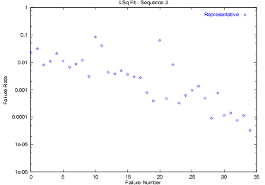
Fitting Example
-
This data shows the failure rate of a program (measured as $1/t$ where $t$ was the length of time the testers were able to run the program before seeing a failure.
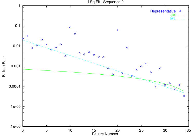
-
Here we have fit this data to the Jelinski-Moranda and Musa Logarithmic models. (Because I have plotted this data using a logarithmic scale for the y-axis, the ML model appears as a straight line in this plot.)
3 Directed Testing
Choose tests designed to reveal
-
many faults
-
as quickly as possible
Choosing Good Test Data
Techniques for selecting directed test data are generally termed either
- white-box, or
- black-box
3.1 Black-Box Testing
Black-box (a.k.a. specification-based) testing chooses tests without consulting the implementation.
- based simply upon our understanding of what the unit is supposed to do.
One of the goals of black-box testing is to be sure that every distinct behavior expected of a unit has been triggered in at least one test. Another is to try to choose tests that are likely to cause trouble, no matter what the actual algorithm is.
Some of the best-known techniques for choosing black-box tests focus on the input values that will be supplied to the unit during testing.
Functional Coverage
a.k.a Equivalence partitioning
-
Choose at least one test that covers each distinct “behavior” described in the requirements.
- Different functions performed by the program
- Different types or ranges of input that get treated or described separately.
- Different types or ranges of output that get treated or described separately.
-
Large, structured projects place emphasis on tracking requirements to functional test cases
Boundary Values Testing
a.k.a., Extremal Values Testing
- Choose as test data the largest and the smallest values for each input and for each “functional” case
- Often misunderstood as simply choosing largest & smallest possible inputs
- Assumes that we have started by attempting functional coverage
Special Values Testing
Choose as test data those certain data values that just tend to cause trouble.
Programmers eventually develop a sense for these. They include
-
For integers: -1, 0, 1
-
For floating point numbers: -e, 0, +e, where “e” is a very small number
-
For strings: the empty string, strings containing only blanks, strings containing no alphabetic characters
What is “Special”?
-
As we move to other data structures, we may develop a suspicion of other special values, e.g.,
- For times of the day: midnight, noon
- For containers of data: an empty container
-
Special values and Boundary values often overlap
-
(F14 example)
3.2 White-Box Testing
White-Box (a.k.a. Implementation-based testing) uses information from the implementation to choose tests.
-
Formally, most white-box testing involves coverage measures, E.g., statement coverage, branch coverage
For example, a common goal in white-box testing is to be sure that every code statement is executed at least once by some test. Another common goal is that, for every conditional branch (ifs, loops, etc.) in the code, that on at least one test that condition will have been true and on at least one test that condition will have been false.
The difficulty with such white-box testing is that it’s almost impossible to be sure you have met one of these goals unless you have special testing software to track the execution of statements and branches over the whole history of testing. Lacking this software, it’s easier to do black-box testing.
-
Informally, design tests specifically to exercise “tricky” parts of the code
However, there is a kind of informal white-box testing that we can do. As programmers, we often write a bit of code and think to ourselves “I wonder if this is really going to work?” That’s a good time to pause and design a test that will check exactly that bit of dicey code.
Common forms:
-
Structural Testing (a.k.a., “path testing” (not per your text)
Designate a set of paths through the program that must be exercised during testing.
- Statement Coverage
- Branch Coverage
- Cyclomatic coverage (“independent path testing”)
- Data-flow Coverage
-
Mutation testing
- Perturbation testing
3.2.1 Statement Coverage
Require that every statement in the code be executed at least once during testing.
Special programs (“software tools”) will monitor this requirement for you.
gprofin GNU gcc/g++ suiteCloverandJaCoCofor Java
Example
cin >> x >> y;
while (x > y)
  {
   if (x > 0)
      cout << x;
   x = f(x, y);
  }
cout << x;
What kinds of tests are required for statement coverage?
3.2.2 Branch Coverage
Requires that every “branch” in the flowchart be tested at least once
- Equivalent to saying that each conditional stmt must be tested as both true and false
- Branch coverage implies Statement Coverage, but not vice versa
  if X < 0 then
    X := -X;
  Y := sqrt(X);
Branch Coverage example
cin >> x >> y;
while (x > y)
  {
   if (x > 0)
      cout << x;
   x = f(x, y);
  }
cout << x;
What kinds of tests are required for branch coverage?
3.2.3 Cyclomatic Coverage
(a.k.a “independent path coverage”, “path testing”)
-
The latter term (used in your text) should be discouraged as it is both vague and means something entirely different to most of the testing community
-
Each independent path must be tested
- An independent path is one that includes a branch not previously taken.
A Control Flow Graph
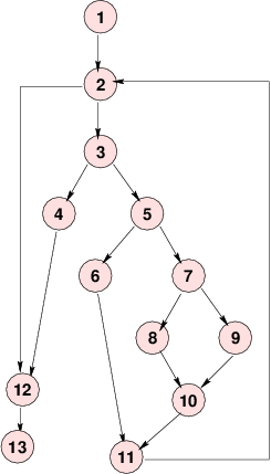 What are the independent paths?
-
1, 2, 3, 4, 12, 13
-
1, 2, 3, 5, 6, 11, 2, 12, 13
- 1, 2, 3, 5, 7, 8, 10, 11, 2, 12, 13
- 1, 2, 3, 5, 7, 9, 10, 11, 2, 12, 13
3.2.4 Cyclomatic Complexity
The number of independent paths in a program can be discovered by computing the cyclomatic complexity (McCabe, 1976)
\[CC(G) = \mbox{Number}(\mbox{edges}) - \mbox{Number}(\mbox{nodes}) + 1\]
-
This is a popular metric for module complexity.
-
Actually pretty trivial: for structured programs with only binary decision constructs, equals number of conditional statements
+1 -
relation to testing is dubious
- simply branch coverage hidden behind smoke and mirrors
Uniqueness
Sets of independent paths are not unique, nor is their size.
-
Earlier we gave this set of 4 paths as a cover
- 1, 2, 3, 4, 12, 13
- 1, 2, 3, 5, 6, 11, 2, 12, 13
- 1, 2, 3, 5, 7, 8, 10, 11, 2, 12, 13
- 1, 2, 3, 5, 7, 9, 10, 11, 2, 12, 13
All are independent.
-
But this set of two paths also covers all
- 1, 2, 3, 5, 6, 11, 2, 3, 5, 7, 8, 10, 11, 2, 3, 5, 7, 9, 10, 11, 2, 12, 13
- 1, 2, 3, 4, 12, 13
And there are no paths independent of these two.
3.2.5 Data-Flow Coverage
Attempts to test significant combinations of branches.
-
Any stmt
iwhere a variableXmay be assigned a new value is called a definition ofXati: def(X,i) -
Any stmt
iwhere a variableXmay be used/retrieved is called a reference or use ofXati: ref(X,i)
def-clear
- A path from stmt
ito stmtjis def-clear with respect to X if it contains no definitions ofXexcept possibly at the beginning (i) and end (j)
all-defs
The all-defs criterion requires that each definition def(X,i) be tested some def-clear path to some reference ref(X,j).
1:  cin >> x >> y;     d(x,1) d(y,1)
2:  while (x > y)      r(x,2), r(y,2)
3:    {
4:     if (x > 0)      r(x,4)
5:        cout << x;   r(x,5)
6:     x = f(x, y);    r(x,6), r(y,6), d(x,6)
7:    }
8:  cout << x;         r(x,8)
What kinds of tests are required for all-defs coverage?
all-uses
The all-uses criterion requires that each pair (def(X,i), ref(X,j)) be tested using some def-clear path from i to j.
1:  cin >> x >> y;     d(x,1) d(y,1)
2:  while (x > y)      r(x,2), r(y,2)
3:    {
4:     if (x > 0)      r(x,4)
5:        cout << x;   r(x,5)
6:     x = f(x, y);    r(x,6), r(y,6), d(x,6)
7:    }
8:  cout << x;         r(x,8)
What kinds of tests are required for all-uses coverage?
3.2.6 Mutation Testing
Given a program \(P\),
-
Form a set of mutant programs that differ from \(P\) by some single change
-
These changes (called mutation operators) include:
- exchanging one variable name by another
- altering a numeric constant by some small amount
- exchanging one arithmetic operator by another
- exchanging one relational operator by another
- deleting an entire statement
- replacing an entire statement by an
abort()call
Mutation Testing (cont.)
-
Run \(P\) and each mutant \(P_i\) on a previously chosen set of tests
-
Compare the output of each \(P_i\) to that of \(P\)
- If the outputs differ on any test, \(P_i\) is killed and removed from the set of mutant programs
- If the outputs are the same on all tests, \(P_i\) is still considered alive.
Mutation Testing (cont.)
A set of test data is considered inadequate if it cannot distinguish between the program as written (\(P\)) and programs that differ from it by only a simple change.
- So if any mutants are still alive after running a set of tests, we augment the tests until we can kill all the mutants.
Mutation Testing Problems
-
Even simple programs yield tens of thousands of mutants. Executing these is time-consuming.
- But most are killed on first few tests
- And the process is automated
-
Some mutants are actually equivalent to the original program:
      ⋮                    ⋮
    X = Y;               X = Y;
    if (X > 0) then      if (Y > 0) then}
      ⋮                    ⋮
- Identifying these can be difficult (and cannot be automated)
3.2.7 Perturbation Testing
Perturbation testing (Zeil) treats each arithmetic expression \(f(\bar{x})\) in the code as if it had been modified by the addition of an error term \(f(\bar{v}) + e(\bar{v})\), where \(v\) are the program variables and \(e\) can be a polynomial of arbitrarily high degree (can approximate almost any error)
-
Monitor the variable values actually encountered during testing
-
Solve for the possible \(e\) functions that would have escaped detection on the tests done so far
- If there are none, we’re done.
- If some exist, can generally be expressed as “coincidental” relations between variables
- e.g., x and y have always been equal in all tests, so substitutions of one for the other could yet not have been detected
3.3 Reliability Modeling with Directed Tests
Most literature on reliability models assumes that it can only be done with representative testing, because
-
Directed tests’ time-to-failure is unrelated to operational time-to-failure
-
Directed tests may find faults “out of order”
Order Statistic Model
Zeil & Mitchell (1996) presented a model for reliability growth under either representative or directed testing.
Assumptions:
-
Software contains \(N\) faults, whose failure rates are described by a distribution \(F\).
-
Faults manifest independently
-
The test process is biased towards finding faults with higher failure rates.
Measurement Process
-
Fault failure rates are measured when the fault has been identified and corrected.
- “post-mortem” analysis
-
Faults are then sorted by failure rate.
-
The sorted data is fitted to an order statistic distribution.
- Order statistics is the study of the probability of selecting certain values when the selection process is biased.
Fitting Example
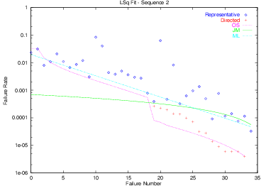
This plot shows an alternative scenario in which the testers started by using representative testing, but once the intervals between failures (and, therefore, between fixes) became lengthy, switched to directed testing to accelerate the process of actually finding and fixing bugs. The Order Statistic model is able, after a period of adjustment to the new testing approach, to model (predict) the severity of the remaining bugs.
1: For some reason, in this field people like to talk about “metrics” rather than the entirely equivalent but less impressive sounding “measures”.