  | 1 of 70


 |   |
| | 1 of 70
| |
We can differentiate testing strategies by overall goal:
Statistical testing
Defect testing
Choosing Test Data
From these motives come different approaches to choosing test data
Representative testing
Directed testing
Choose data that is representative of the way the end users will exercise the software.
Producing Representative Tests
Test data can be obtained via
Producing Representative Tests
Test data can be obtained via
collected data from an existing system
Producing Representative Tests
Test data can be obtained via
collected data from an existing system
further selection may be needed
Producing Representative Tests
Test data can be obtained via
collected data from an existing system
further selection may be needed
cannot accomodate new functionality
Producing Representative Tests
Test data can be obtained via
collected data from an existing system
further selection may be needed
cannot accomodate new functionality
random generators
Producing Representative Tests
Test data can be obtained via
collected data from an existing system
further selection may be needed
cannot accomodate new functionality
random generators
non-uniform, to match desired distribution
Producing Representative Tests
Test data can be obtained via
collected data from an existing system
further selection may be needed
cannot accomodate new functionality
random generators
non-uniform, to match desired distribution
can be hard to generate non-numeric ADT values
Representative Testing
The operational profile is a description of the probability distribution of the input.
It describes how often, during operational program use, certain “kinds” of inputs will be seen.
Sample Op Profile
| Input Category | Percentage | |
|---|---|---|
| Transaction Proc. | 85% | |
| Balancing | 14% | |
| Year-end Report | 1% | |
For an accounting program, we might start with an observation that past activities have broken down like this.
Sample Op Profile
| Input Category | Percentage | |
|---|---|---|
| Transaction Proc. | 85% | |
| Balancing | 14% | |
| Year-end Report | 1% | |
For an accounting program, we might start with an observation that past activities have broken down like this.
Sample Op Profile
| Input Category | Percentage | |
|---|---|---|
| Transaction Proc. | 85% | |
| New account | 7% | |
| Close account | 3% | |
| Debits | 70% | |
| Credits | 20% | |
| Balancing | 14% | |
| Year-end Report | 1% | |
Sample Op Profile
| Input Category | Percentage | |
|---|---|---|
| Transaction Proc. | 85% | |
| New account | 7% | |
| Close account | 3% | |
| Debits | 70% | |
| Credits | 20% | |
| Balancing | 14% | |
| Year-end Report | 1% | |
Sample Op Profile
| Input Category | Percentage | ||
|---|---|---|---|
| Transaction Proc. | 85% | ||
| New account | 7% | ||
| new | 90% | ||
| already exists | 10% | ||
| Close account | 3% | ||
| non-existent | 15% | ||
| exists | 85% | ||
| Debits | 70% | ||
| non-existent | 25% | ||
| exists | 75% | ||
| Credits | 20% | ||
| non-existent | 25% | ||
| exists | 75% | ||
| Balancing | 14% | ||
| Year-end Report | 1% | ||
Representative testing difficulties
Uncertainty in the operational profile
High costs of generating the operational profile
Statistical uncertainty
A growth model is a mathematical model of the system reliability change as it is tested and faults are removed
Used as a means of reliability prediction by extrapolating from current data
Reliability modeling procedure
Determine operational profile of the software
Generate a set of test data corresponding to the profile
Apply tests, measuring amount of execution time between each failure
After a statistically valid number of tests have been executed, reliability can be measured
Reliability metrics
Some common metrics1 that come out of these statistical models are:
Probability of failure on demand
POFOD = 0.001 means 1 out of 1000 service requests result in failureRate of fault occurrence (ROCOF)
ROCOF = 0.02 means 2 failures are likely in each 100 operational time unitsReliability metrics
Mean time to failure
MTTF = 500 means that the average time between failures is 500 time unitsAvailability
Avail = 0.998 means software is available for 998 out of 1000 time unitsMeasure the number of system failures for a given number of system inputs
POFODMeasure the time (or number of transactions) between system failures
ROCOF and MTTFMeasure the time to restart after failure
AvailTime units
Time units in reliability measurement must be carefully selected. Not the same for all systems
Raw execution time (for non-stop systems)
Calendar time (for systems which have a regular usage pattern e.g. systems which are always run once per day)
Number of transactions (for systems which are used on demand)
Assumptions:
Software contains \(N\) faults (\(N\) is unknown)
Each fault manifests (causes a failure) at rate \(\phi\)
Faults manifest independently
Faults are fixed perfectly, without introducing new ones
If we have repaired \(i\) faults, the program’s failure rate \(\lambda\) is \[ \lambda_{i} = (N-i)\phi \]
Observed reliability growth
Simple equal-step model but does not reflect reality
Reliability does not necessarily increase with change as the change can introduce new faults
The rate of reliability growth tends to slow down with time as frequently occurring faults are discovered and removed from the software
Assumptions:
Software can never be completely free of faults.
Faults manifest independently
Faults are found in decreasing order of failure rate.
The program failure rate before repairing any faults is \(\lambda_{0}\)
Faults are fixed perfectly, without introducing new ones
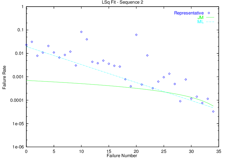
If we have repaired \(i\) faults, the program’s failure rate \(\lambda\) is \[ \lambda_{i} = \lambda_{0} e^{-\theta i} \]
Fitting Example
Each point represents a failed test (after which the software was debugged and fixed).
Choosing Good Test Data
Techniques for selecting directed test data are generally termed either
Black-box (a.k.a. specification-based) testing chooses tests without consulting the implementation.
Functional Coverage
a.k.a Equivalence partitioning
Choose at least one test that covers each distinct “behavior” described in the requirements.
Large, structured projects place emphasis on tracking requirements to functional test cases
Boundary Values Testing
a.k.a., Extremal Values Testing
Special Values Testing
Choose as test data those certain data values that just tend to cause trouble.
Programmers eventually develop a sense for these. They include
For integers: -1, 0, 1
For floating point numbers: -e, 0, +e, where “e” is a very small number
For strings: the empty string, strings containing only blanks, strings containing no alphabetic characters
What is “Special”?
As we move to other data structures, we may develop a suspicion of other special values, e.g.,
Special values and Boundary values often overlap
(F14 example)
White-Box (a.k.a. Implementation-based testing) uses information from the implementation to choose tests.
Common forms:
Structural Testing (a.k.a., “path testing” (not per your text)
Designate a set of paths through the program that must be exercised during testing.
Mutation testing
Require that every statement in the code be executed at least once during testing.
Special programs (“software tools”) will monitor this requirement for you.
gprof in GNU gcc/g++ suiteClover and JaCoCo for JavaExample
cin >> x >> y;
while (x > y)
  {
   if (x > 0)
      cout << x;
   x = f(x, y);
  }
cout << x;
What kinds of tests are required for statement coverage?
Requires that every “branch” in the flowchart be tested at least once
  if X < 0 then
    X := -X;
  Y := sqrt(X);
Branch Coverage example
cin >> x >> y;
while (x > y)
  {
   if (x > 0)
      cout << x;
   x = f(x, y);
  }
cout << x;
What kinds of tests are required for branch coverage?
(a.k.a “independent path coverage”, “path testing”)
The latter term (used in your text) should be discouraged as it is both vague and means something entirely different to most of the testing community
Each independent path must be tested
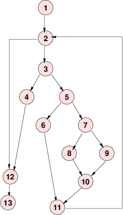
A Control Flow Graph
 What are the independent paths?
A Control Flow Graph
What are the independent paths?
1, 2, 3, 4, 12, 13
A Control Flow Graph
What are the independent paths?
1, 2, 3, 4, 12, 13
1, 2, 3, 5, 6, 11, 2, 12, 13
A Control Flow Graph
What are the independent paths?
1, 2, 3, 4, 12, 13
1, 2, 3, 5, 6, 11, 2, 12, 13
A Control Flow Graph
What are the independent paths?
1, 2, 3, 4, 12, 13
1, 2, 3, 5, 6, 11, 2, 12, 13
The number of independent paths in a program can be discovered by computing the cyclomatic complexity (McCabe, 1976)
\[CC(G) = \mbox{Number}(\mbox{edges}) - \mbox{Number}(\mbox{nodes}) + 1\]
This is a popular metric for module complexity.
Actually pretty trivial: for structured programs with only binary decision constructs, equals number of conditional statements +1
relation to testing is dubious
Uniqueness
Sets of independent paths are not unique, nor is their size.
Uniqueness
Sets of independent paths are not unique, nor is their size.
Earlier we gave this set of 4 paths as a cover
Uniqueness
Sets of independent paths are not unique, nor is their size.
Earlier we gave this set of 4 paths as a cover
Uniqueness
Sets of independent paths are not unique, nor is their size.
Earlier we gave this set of 4 paths as a cover
Uniqueness
Sets of independent paths are not unique, nor is their size.
Earlier we gave this set of 4 paths as a cover
Uniqueness
Sets of independent paths are not unique, nor is their size.
Earlier we gave this set of 4 paths as a cover
All are independent.
Uniqueness
Sets of independent paths are not unique, nor is their size.
Earlier we gave this set of 4 paths as a cover
All are independent.
But this set of two paths also covers all
Uniqueness
Sets of independent paths are not unique, nor is their size.
Earlier we gave this set of 4 paths as a cover
All are independent.
But this set of two paths also covers all
Uniqueness
Sets of independent paths are not unique, nor is their size.
Earlier we gave this set of 4 paths as a cover
All are independent.
But this set of two paths also covers all
And there are no paths independent of these two.
Attempts to test significant combinations of branches.
Any stmt i where a variable X may be assigned a new value is called a definition of X at i: def(X,i)
Any stmt i where a variable X may be used/retrieved is called a reference or use of X at i: ref(X,i)
def-clear
i to stmt j is def-clear with respect to X if it contains no definitions of X except possibly at the beginning (i) and end (j)all-defs
The all-defs criterion requires that each definition def(X,i) be tested some def-clear path to some reference ref(X,j).
1:  cin >> x >> y;     d(x,1) d(y,1)
2:  while (x > y)      r(x,2), r(y,2)
3:    {
4:     if (x > 0)      r(x,4)
5:        cout << x;   r(x,5)
6:     x = f(x, y);    r(x,6), r(y,6), d(x,6)
7:    }
8:  cout << x;         r(x,8)
What kinds of tests are required for all-defs coverage?
all-uses
The all-uses criterion requires that each pair (def(X,i), ref(X,j)) be tested using some def-clear path from i to j.
1:  cin >> x >> y;     d(x,1) d(y,1)
2:  while (x > y)      r(x,2), r(y,2)
3:    {
4:     if (x > 0)      r(x,4)
5:        cout << x;   r(x,5)
6:     x = f(x, y);    r(x,6), r(y,6), d(x,6)
7:    }
8:  cout << x;         r(x,8)
What kinds of tests are required for all-uses coverage?
Given a program \(P\),
Form a set of mutant programs that differ from \(P\) by some single change
These changes (called mutation operators) include:
abort() callMutation Testing (cont.)
Run \(P\) and each mutant \(P_i\) on a previously chosen set of tests
Compare the output of each \(P_i\) to that of \(P\)
Mutation Testing (cont.)
A set of test data is considered inadequate if it cannot distinguish between the program as written (\(P\)) and programs that differ from it by only a simple change.
Mutation Testing Problems
Even simple programs yield tens of thousands of mutants. Executing these is time-consuming.
Some mutants are actually equivalent to the original program:
      ⋮                    ⋮
    X = Y;               X = Y;
    if (X > 0) then      if (Y > 0) then}
      ⋮                    ⋮
Perturbation testing (Zeil) treats each arithmetic expression \(f(\bar{x})\) in the code as if it had been modified by the addition of an error term \(f(\bar{v}) + e(\bar{v})\), where \(v\) are the program variables and \(e\) can be a polynomial of arbitrarily high degree (can approximate almost any error)
Monitor the variable values actually encountered during testing
Solve for the possible \(e\) functions that would have escaped detection on the tests done so far
Most literature on reliability models assumes that it can only be done with representative testing, because
Directed tests’ time-to-failure is unrelated to operational time-to-failure
Directed tests may find faults “out of order”
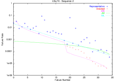
Order Statistic Model
Zeil & Mitchell (1996) presented a model for reliability growth under either representative or directed testing.
Assumptions:
Software contains \(N\) faults, whose failure rates are described by a distribution \(F\).
Faults manifest independently
The test process is biased towards finding faults with higher failure rates.
Measurement Process
Fault failure rates are measured when the fault has been identified and corrected.
Faults are then sorted by failure rate.
The sorted data is fitted to an order statistic distribution.
Fitting Example
1: For some reason, in this field people like to talk about “metrics” rather than the entirely equivalent but less impressive sounding “measures”.
| | 1 of 70
| |