


The Algebra of Big-O
Steven J. Zeil
In the previous lesson we saw the definition of “time proportional to” (big-O), and we saw how it could be applied to simple algorithms. I think you will agree with me that the approach we took was rather tedious, and probably you wouldn’t want to use it in practice.
We are going to start working towards more usable approach to match the complexity of algorithm. We will start by looking at rather peculiar algebraic rules that can be applied for manipulating big-O expressions. In the next lesson, we shall then look at the process of taking an algorithm the way you and I actually write it in typical programming languages and analyzing that to produce the original big-O expressions.
For now, though, let us start by discussing how we might manipulate big-O expressions once we’ve actually got them. The first thing we have to do is to recognize that the algebra of big-O expressions is not the same “good old fashioned” algebra you learned back in high school. The reason is that when we say something like $O(f(N)) = O(g(N))$, we are not comparing two numbers to one another with that ‘=’, nor are we claiming that f(N) and g(N) are equal. We are instead comparing two sets of programs (or functions describing the speed of programs) and we are stating that any program in the set $O(f(N))$ is also in the set $O(g(N))$ and vice-versa.
We will now explore the peculiar algebra of big-O, and, through that algebra, will see why big-O is appropriate for comparing algorithms.
1 Basic Manipulation
We start with a pair of simple, almost self-evident rules:
Algebraic Rule 1: $f(\bar{n}) + g(\bar{n}) \in O(f(\bar{n}) + g(\bar{n}))$
This rule comes into play most often when we discover that a program has to do two (or more) things before it is finished, one of which takes time $f(\bar{n})$ and the other takes time $g(\bar{n})$. The rule simply says that the running time of the entire program might be no faster than the sum of the running times of its constituent parts.
Because this is only an upper bound, the program might actually be faster than that (e.g., if the first part of the program prepares the data in some fashion that allows the second part to run faster than it would have in isolation). But it will be no slower, in the worst case, than some constant times the sum of the two run time bounds.
Algebraic Rule 2: $f(\bar{n}) * g(\bar{n}) \in O(f(\bar{n}) * g(\bar{n}))$
This rule comes into play most often when we discover that a program has a loop that runs through $f(\bar{n})$ iterations, and each iteration of the loop takes $O(g(\bar{n}))$ time. Then the program will be no slower, in the worst case, than some constant times the product of those two functions.
2 Dropping Constant Multipliers
Our next rule is a bit less intuitive:
- Algebraic Rule 3:
- $O(c*f(\bar{n})) = O(f(\bar{n}))$
This rule suggests that, for sufficiently large $\bar{n}$, constant multipliers “don’t count”.
2.1 Intuitive Justification
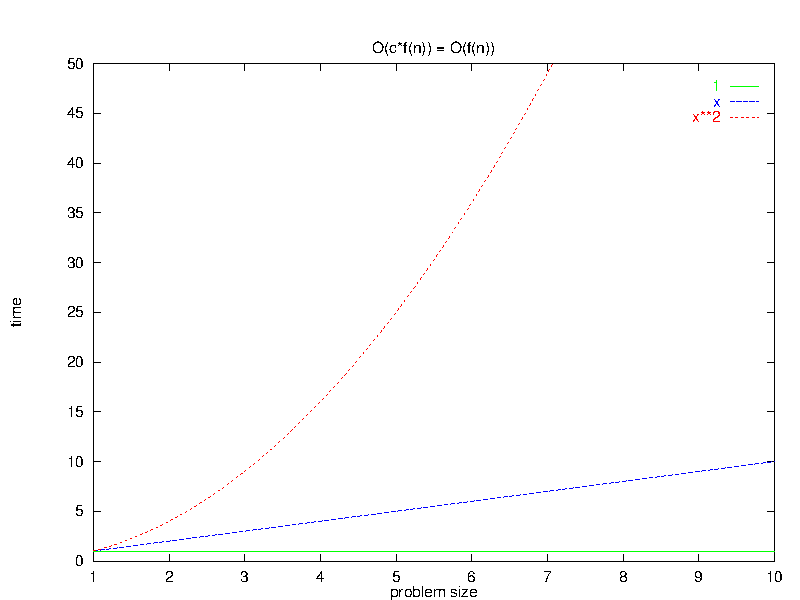
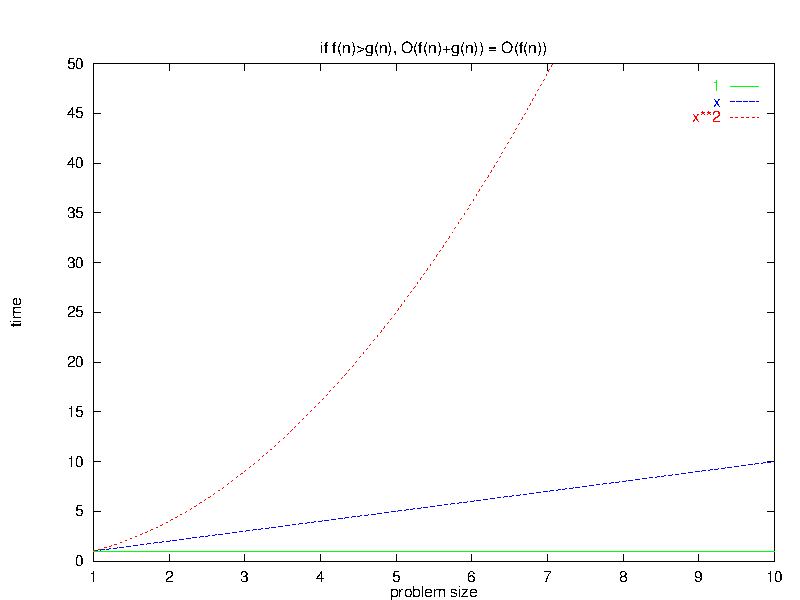
To see why this might be so, suppose we have three programs that run in time $O(1)$, $O(x)$, and $O(x^{2})$, where $x$ is the size of the input set.
Notice from the plot of these three times, that, for sufficiently large $x$, the $O(x)$ time falls between the other two.
  | 1 of 6 |   |
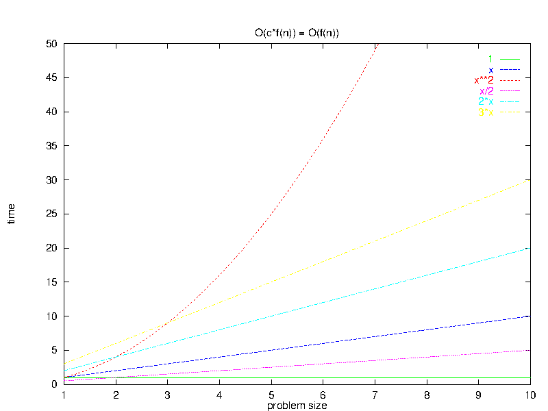
2.1.1 So What Good are Constants?
Does this mean that constant multipliers aren’t relevant at all?
-
No. Suppose we had two programs A and B with times \[ t_{A} (N) = N * (1 second) \] \[ t_{B} (N) = N * (1 minute) \]
-
For $N=60$, this is the difference between waiting 1 minute and waiting for 1 hour. No one will argue that this difference is insignificant.
-
-
But now suppose that we consider a third program C with an even smaller constant:
\[ t_{C} (N) = N^{2} * (0.01 second) \]
Even though this program has a much smaller constant factor, and will perform much faster on small $N$, it will be slower than program $A$ whenever $N > 100$ and slower than $B$ when $N > 6000$.
-
So the constant can play a role in choosing the faster algorithm only when the function parts of the complexity are equal.
2.2 Proof: $O(c*f(\bar{n})) = O(f(\bar{n}))$
All we have done so far is to give examples that this rule holds. No number of examples can constitute a proof. To prove that it holds in general, consider any program with running time $t(\bar{n}) = O(c*f(\bar{n}))$.
By the definition of $O(\ldots )$, we have:
\[ \exists c_1, \bar{n}_0 | \bar{n} > \bar{n}_0 \Rightarrow t(\bar{n}) \leq c_1 (c * f(\bar{n})) \]
But, grouping the multiplication slightly differently gives
\[ \exists c_1, \bar{n}_0 | \bar{n} > \bar{n}_0 \Rightarrow t(\bar{n}) \leq (c_1 * c) f(\bar{n}) \]
Now, since $c$ and $c_{1}$ are both constants, we can introduce a new constant $c_{2}$:
\[ c_{2} = c_{1} * c \]
and then we can claim that
\[ \exists c_1, \bar{n}_0 | \bar{n} > \bar{n}_0 \Rightarrow t(\bar{n}) \leq c_2 * f(\bar{n}) \]
But this is just the definition of $O(f(\bar{n}))$, so we conclude that
\[ t(\bar{n})=O(f(\bar{n})) \]
Therefore any program in $O(c*f(\bar{n}))$ is also in $O(f(\bar{n}))$.
It’s easy enough to modify the above argument to show that any program in $O(f(\bar{n}))$ is also in $O(c*f(\bar{n}))$ (e.g., replace $c$ by $1/c$).
So the sets $O(f(N))$ and $O(c*f(N))$ are, in fact, the same.
Q.E.D.
This rule can be applied across sums, by the way. If we have two functions f(N) and g(N) and two constants $c_1$ and $c_2$, then it’s easy to modify the above proof to show that
\[O(c_1*f(\bar{n}) + c_2*f(\bar{n})) = O(f(\bar{n}) + g(\bar{n}))\]
3 Larger Terms Dominate a Sum
Algebraic Rule 4:If $\exists \bar{n}_0 \; | \; \forall \bar{n} > \bar{n}_0, \, f(\bar{n}) \geq g(\bar{n})$, then $O(f(\bar{n}) + g(\bar{n})) = O(f(\bar{n}))$
This rule states that, if we have a program that does two different things before it finishes, then for large input sets the slower of these two will dominate the overall time.
3.1 Intuitive Justification
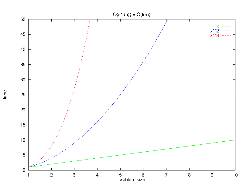
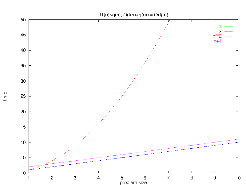
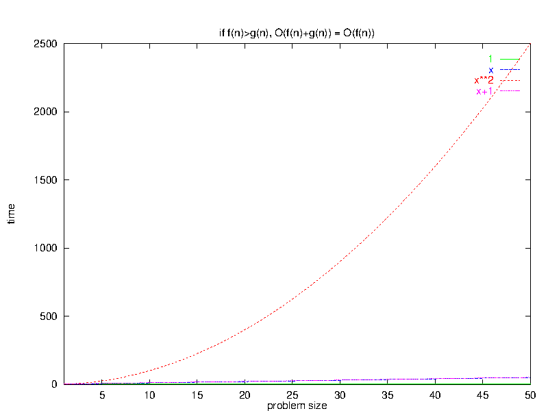
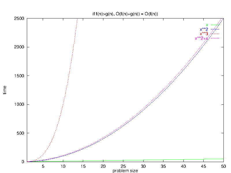
To see why this might be so, suppose we have three programs that run in time $O(1)$, $O(x)$, and $O(x^{2})$, where $x$ is the size of the input set.
As before, we note that, for sufficiently large $x$, the $O(x)$ time falls between the other two.

| | 1 of 6 | |
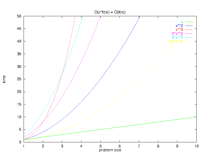
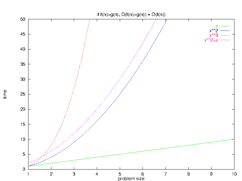
In essence, adding a “lower-order” function (e.g., $x$) to a “higher-order” one (e.g., $x^{2}$) does not sufficiently alter the curvature of the new higher-order function enough to change its big-O relationship to other even higher- (e.g., $x^{3}$) and lower-order (e.g., $x$) functions.
3.2 Proof: Larger Terms Dominate a Sum
To prove that, if $\forall \bar{n} > \bar{n}_0. f(\bar{n}) \geq g(\bar{n})$, then $O(f(\bar{n}) + g(\bar{n})) = O(f(\bar{n})),$ consider any program with running time $t(\bar{n}) = O(f(\bar{n}) + g(\bar{n}))$.
By the definition of big-O, we know that, for some $c$ and $\bar{n}_1$, we have:
\[ \bar{n} > \bar{n}_1 \Rightarrow t(\bar{n}) \leq c (f(\bar{n}) + g(\bar{n})) \]
But assume that $\forall \bar{n} >{} 0, f(\bar{n}) \geq g(\bar{n})$
Then we can claim that the following are also true:
\[ \begin{align} \bar{n} > \max(\bar{n}_0, \bar{n}_1) & \Rightarrow t(\bar{n}) \leq c (f(\bar{n}) + g(\bar{n}) ) \;\;\; & (1)\\ \bar{n} > \max(\bar{n}_0, \bar{n}_1) & \Rightarrow f(\bar{n}) > g(\bar{n}) & (2) \end{align} \]
But equation (2) suggests that we can, for those values of $\bar{n}$, replace the $g(\bar{n})$ by $f(\bar{n})$ in equation (1) and, because we are replacing one quantity by an even larger one, the “$\leq$” relation will still hold:
\[ \begin{eqnarray} \bar{n} > \max(\bar{n}_0, \bar{n}_1) & \Rightarrow & t(\bar{n}) \leq c (f(\bar{n}) + f(\bar{n})) \\ \bar{n} > \max(\bar{n}_0, \bar{n}_1) & \Rightarrow & t(\bar{n}) \leq 2c * f(\bar{n}) \end{eqnarray} \]
But $2c$ and $max(\bar{n}_{0}, \bar{n}_{1})$ are just constants, so that final
equation simply expresses the big-O definition: $t(\bar{n}) = O(f(\bar{n}))$
Q.E.D.
4 Logarithms are Fast
Our final rule doesn’t come into play as often as the others, but is still useful on occasion:
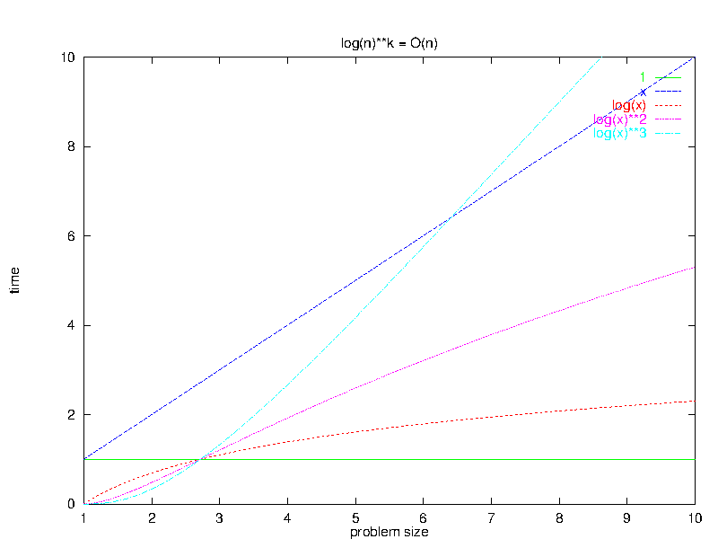
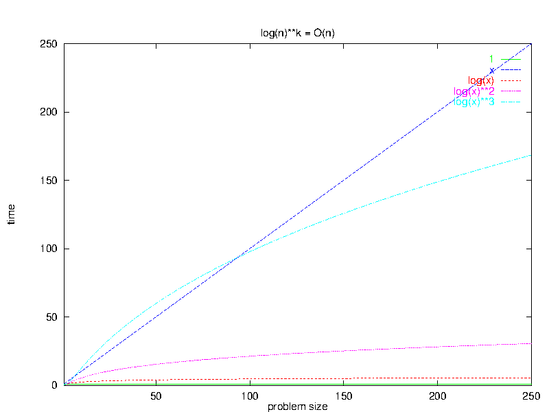
Algebraic Rule 5: $\forall k \geq 0, O(\log^{k}(n)) \subset O(n)$
Remember that big-O expressions are really describing sets of functions, so the $\subset$ in this rule says that logarithms are faster than linear functions.
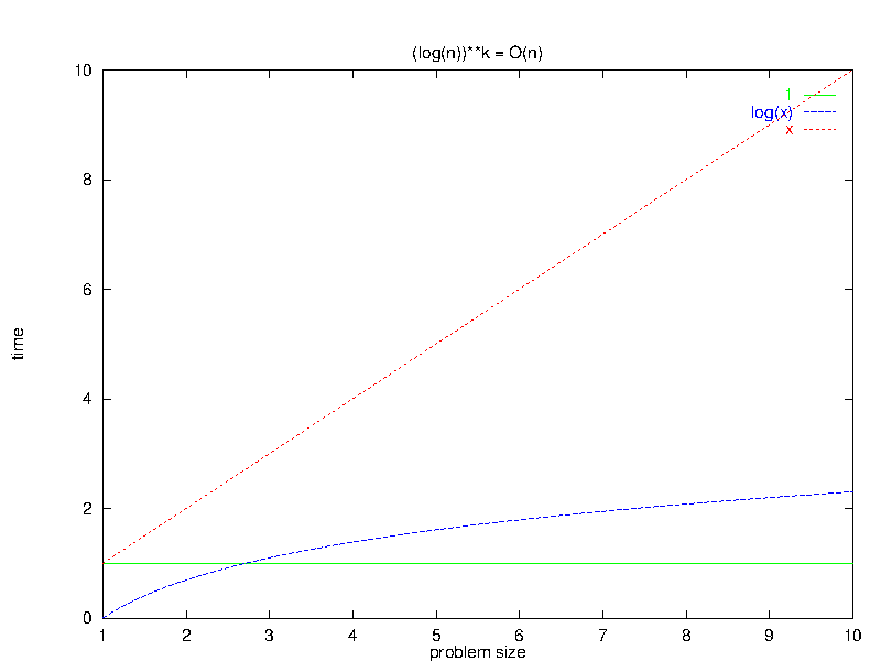
The best time we could ask for from any algorithm is $O(1)$, meaning that the algorithm never exceeds some constant run time, no matter how large the input set.
An algorithm that works in logarithmic time is often nearly as good as one that works in constant time.
Notice how the tail of the log curve bends over nearly horizontally, almost but not quite ever becoming parallel to the flat $O(1)$ plot.
So $O(\log N)$ is just slightly slower, for large $N$, than $O(1)$ and significantly faster than $O(N)$.
| | 1 of 3 | |
5 Summary of big-O Algebra
The five rules we have presented:
-
$f(\bar{n}) + g(\bar{n}) \in O(f(\bar{n}) + g(\bar{n}))$
-
$f(\bar{n}) * g(\bar{n}) \in O(f(\bar{n}) * g(\bar{n}))$
-
$O(c*f(\bar{n})) = O(f(\bar{n}))$
-
If $\exists n_0 | \forall \bar{n} > n_0, f(\bar{n}) \geq g(\bar{n})$, then $O(f(\bar{n}) + g(\bar{n})) = O(f(\bar{n}))$
-
$\forall k \geq 0, O(\log^{k}(n)) \subset O(n)$
allow us to simplify complicated analyses without resorting to a full-blown proof based upon the definition of big-O.
For example, we earlier looked at a piece of code that we felt ran in time
\[ \begin{eqnarray*} t(N) & = & N^{2} (2t_{\mbox{asst}} + t_{\mbox{comp}} + 4t_{\mbox{add}} + 3t_{\mbox{mult}}) \\ & & + N (3t_{\mbox{asst}} + 2t_{\mbox{comp}} + 2t_{\mbox{add}} + t_{\mbox{mult}}) \\ & & + 1 (t_{\mbox{asst}} + t_{\mbox{comp}}) \end{eqnarray*} \]
Since this is the exact running time, it is also an upper bound. Therefore,
\[ \begin{eqnarray*} t(N) & \in & O(N^{2} (2t_{\mbox{asst}} + t_{\mbox{comp}} + 4t_{\mbox{add}} + 3t_{\mbox{mult}}) \\ & & + N (3t_{\mbox{asst}} + 2t_{\mbox{comp}} + 2t_{\mbox{add}} + t_{\mbox{mult}}) \\ & & + 1 (t_{\mbox{asst}} + t_{\mbox{comp}})) \end{eqnarray*} \]
By rule 4, the higher-order $N^{2}$ term will dominate this sum:
\[ t(N) \in O(N^{2} (2t_{\mbox{asst}} + t_{\mbox{comp}} + 4t_{\mbox{add}} + 3t_{\mbox{mult}}))\]
By rule 3, we can discard the constant multipliers:
\[ t(N) \in O(N^{2}) \]
This is, I hope you’ll agree, much simpler than the proof we engaged in when we first analyzed that code.
5.1 The Tao of N
Finally, keep in mind that $n$ or $N$ is merely a placeholder here for what may be an expression involving multiple measures of the input set size. Only the last of these rules is limited to a single variable (because the expression “$\log(n)$” only makes sense if $n$ is a single quantity, although it can still be any single expression, e.g., $\log(n^{3} + 1/n)$.
For example, if we were presented with a function that was $O(30.0 x^{2} + 15.0 y + 2 x)$, we could simplify it as follows:
\[\begin{align*} O(30.0 x^{2} + 15.0 y + 2 x) & \\ & = O(30.0 x^{2} + 15.0y) & \mbox{(by rule 4)} \\ & = O(x^{2} + y) & \mbox{(by rule 3)} \end{align*}\]
and would have to stop there. Although $x^{2}$ has a larger exponent than $y$, we can’t assume that it dominates $y$ unless we have some other information about the relative sizes of $x$ and $y$.
If someone were to come by later and inform us, “Oh, by the way, it’s always true that $y \leq x$”, then we could indeed simplify the above to $O(x^{2})$. On the other hand, if that same mysterious font of information were to instead say, “Oops, my mistake. Actually $y \geq x^{3}$”, then we would simplify $O(x^{2} + y)$ to $O(y)$.
6 Always Simplify!
Whenever you analyze an algorithm in an assignment, quiz or exam in this course, you should employ these algebraic rules to present your answer in the simplest form possible. If you don’t, your answer will be considered wrong!