  | 1 of 19


 |   |
| | 1 of 19
| |
OK, we’ve got our hash functions. They’re not perfect, so we can expect collisions. How do we resolve these collisions?
There are two general approaches:
Open Hashing: The hash table performs as an “index” to a set of structures that hold multiple items.
Closed Hashing: The keys are stored in the table itself, so we have to search for an open slot within the table.
Historically, one of the most common approaches to dealing with collisions has been to use fixed size buckets, e.g., an array that can hold up to k (some small constant) elements.
The problem with this is that if we get more than k collisions at the same location, we still need to fall back to some other scheme.
So instead, we’ll look at separate chaining, in which the hash table is implemented as an array of variable sized containers that can hold however many elements that have actually collided at that location.
template <class T,
          int hSize,
          class HashFun,
          class CompareEQ=equal_to<T> >
class hash_set
{
    typedef list<T> Container;

public:
  hash_set (): buckets(hSize), theSize(0)
   {}
    ⋮
private:
  vector<Container> buckets;
  HashFun hash;
  CompareEQ compare;
  int theSize;
};
We’ll illustrate separate chaining as a vector of linked lists of elements.
This template takes more parameters than usual. The purpose of the parameters T and hSize should be self-evident.
HashFun is a functor class used to provide the hash function hash.
CompareEQ is another functor class, used to provide an equality comparison (like the less-than comparators used in std::set and std::map). This defaults to the std functor class equal_to, which uses the T class’s == operator.
private:

  Container& bucket (const T& element)
    {
      return buckets[hash(element) % Size];
    }
This utility function locates the list that will contain a given element, if that element really is somewhere in the table.
Now we use the bucket() function to implement the set count() function.
int count (const T& element) const
  {
    const Container& theBucket = bucket(element);
    return (find_if(theBucket.begin(),
                    theBucket.end(),
                    bind1st(compare, element))
            == theBucket.end()) ? 0 : 1;
  }
First we use bucket() to find the list where this element would be. Then we search the list for an item equal to element.
The insert code is quite similar.
void insert (const T& element)
  {
    Container& theBucket = bucket(element);
    Container::iterator pos =
      find_if(theBucket.begin(), theBucket.end(),
                    bind1st(compare, element));
    if (pos == theBucket.end())
      {
        theBucket.push_back(element);
        ++theSize;
      }
    else
      *pos = element;
  }
We use bucket() to find the list, then search the list for the element we want to insert. If it’s already in there, we replace it. If not, we add it to the list.
And erase follows pretty much the same pattern.
void erase (const T& element)
  {
    Container& theBucket = bucket(element);
    Container::iterator pos =
      find_if(theBucket.begin(), theBucket.end(),
                    bind1st(compare, element));
    if (pos != theBucket.end())
      {
        theBucket.erase(pos);
        --theSize;
      }
  }
For example, suppose that we wished to insert the strings
Adams, Baker, Clarke, Doe, Evans
into a hash structure using an array size of 7 and, for the sake of example, a terrible hash function that simply uses the size of the strings.
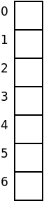
We start with an array of empty linked list headers.
Our first input, “Adams”, according to our bad hash function, hashes to location 5.
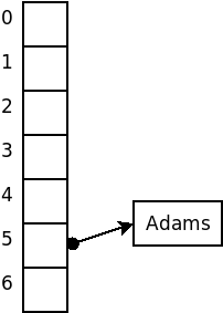
So we add “Adam” to the linked list in position 5 of our array.
Our next input is “Baker”, which also hashes to position 5.
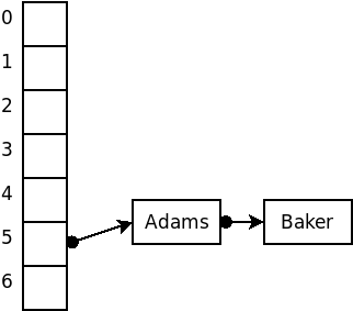
So we add “Baker” to the same list containing “Adam”.
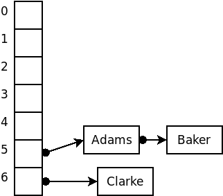
“Clarke”, however, hashes to position 6. So it goes into a new list at position 6.
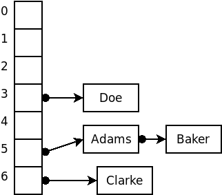
Similarly, “Doe” hashes to position 3. So it goes into a new list at position 3.
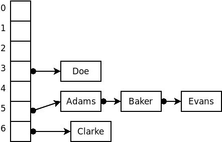
Finally, “Evans” hashes to position 5. So it goes into the existing list at position 5.
  | 1 of 6 |   |
The code discussed here is available as an animation that you can run to see how it works. (This demo deliberately uses an awful hash function, the length of the string, so that you will have a chance to see lots of collisions taking place.)
You might take note that, as the chains grow longer, the search times become more “sequential search” like. Of course, if we increased the table size, we would hope that the data elements would be dispersed across the larger table, making the average list length shorter. So there is a very direct tradeoff here between memory use (table size) and speed.
Suppose we have inserted $N$ items into a table of size hSize.
In the worst case, all $N$ items will hash to the same list, and we will be reduced to doing a linear search of that list: $O(N)$. (Your text uses sets instead of lists for the buckets, which would reduce this cost to $O(\log N)$.) On the other hand, the use of sets requires that the data elements support a < comparison instead of (or in addition to) the == comparison required with list buckets.
In the average case, we assume that the N items are distributed evenly among the lists. Since we have N items distributed among hSize lists, we are looking at $O\left(\frac{N}{\mbox{hSize}}\right)$.
If hsize is much larger than N, and if our hash function uniformly distributes our keys, then most lists will have 0 or 1 item, an the average case would be approximately $O(1)$. But if $N$ is much larger than hSize, we are looking at an $O(N)$ linear search sped up by a constant factor (hSize), but still $O(N)$. So hash tables let us trade space for speed.
In closed hashing, the hash array contains individual elements rather than a collection of elements. When a key we want to insert collides with a key already in the table, we resolve the collision by searching for another open slot within the table where we can place the new key.
enum HashStatus { Occupied, Empty, Deleted };

template <class T>
struct HashEntry
{
  T data;
  HashStatus info;

  HashEntry(): info(Empty)  {}
  HashEntry(const T& v, HashStatus status)
    : data(v), info(status) {}

};
Each slot in the hash table contains one data element and a status field indicating whether that slot is occupied, empty, or deleted.
template <class T, int hSize, class HashFun,
          class CompareEQ=equal_to<T> >
class hash_set
{
public:
  hash_set (): table(hSize), theSize(0)
    {}
   ⋮
private:

  int find (const T& element, int h0) const
   ⋮

  vector<HashEntry<T> > table;
  HashFun hash;
  CompareEQ compare;
  int theSize;
};
The hash table itself consists of a vector/array of these HashEntry elements.
Collisions are resolved by trying a series of locations, $h_{\mbox{0}}$, $h_{\mbox{1}}$, $h_{\mbox{hSize-1}}$, until we find what we are looking for. These locations are given by
\[ h_{i}(\mbox{key}) = (\mbox{hash}(\mbox{key}) + f(i)) % \mbox{hSize} \]
where $f$ is some integer function, with $f(0)=0$. We’ll look at what makes a good $f$ in a little bit.
With these locations, the basic idea is
Searching: try cells $h_{i}(\mbox{key}), i=0, 1, \ldots$ until we find the key we want or an empty slot.
Inserting: try cells $h_{i}(\mbox{key}), i=0, 1, \ldots$ until we find the same key, an empty slot, or a deleted slot. Put the new key there, and mark the slot “occupied”.
Erasing: try cells $h_{i}(\mbox{key}), i=0, 1, \ldots$ until we find the key we want or an empty slot. If we find the key, mark that slot as “deleted”.
Here’s a “utility” search function for use with closed hashing. It takes as parameters the element to search for and the hash value of that element.
int find (const T& element, int h0) const
{
 unsigned h = h0 % hSize;
 unsigned count = 0;
 while ((table[h].info == Deleted ||
   (table[h].info == Occupied
    && (!compare(table[h].data, element))))
    && count < hSize)
   {
     ++count;
     h = (h0 + f(count)) % hSize;
   }
 if (count >= hSize
     || table[h].info == Empty)
    return hSize;
 else
    return h;
}
The loop condition is fairly complicated and bears discussion. There are three ways to exit this loop:
If we hit an “Empty” space (i.e., not “Deleted”, and not “Occupied”)
If we hit an “Occupied” space that has the key we’re looking for
If we have tried hSize different positions. (There’s no place else to look!)
With that utility, search operations like the set count() are easy. We simply compute the hash value and then call find. Then we check to see if the element was found or not.
int count (const T& element)
{
  unsigned h0 = hash(element);
  unsigned h = find(element, h0);
  return  (h != hSize) ? 1 : 0;
}
void erase (const T& element)
{
  unsigned h0 = hash(element);
  unsigned h = find(element, h0);
  if (h != hSize)
    table[h].info = Deleted;
}
The code to remove elements is just as simple. We compute the hash function and try to find that element. If it’s found, we mark that slot “Deleted”.
Inserting is a bit more complicated.
bool insert (const T& element)
{
  unsigned h0 = hash(element);
  unsigned h = find(element, h0);      ➀
  if (h == hSize) {
    unsigned count = 0;
    h = h0;
    while (table[h].info == Occupied    ➁
           && count < hSize)
      {
        ++count;
        h = (h0 + f(count)) % hSize;
      }
    if (count >= hSize)
      return false;  // could not add
    else
      {
        table[h].info = Occupied;
        table[h].data = element;
        return true;
      }
  }
  else { // replace
    table[h].data = element;
    return true;
  }
}
➀ Because this is a set (and not a multiset) we first do an ordinary search to see if the element is already there.
➁ If not, we need to find a place to put it. The loop that does this looks a lot like the find loop, but unlike find, we stop at the first “Deleted” or “Empty” slot.
In the other searches, we had kept going past “Deleted” slots, because the element we wanted might have been stored after an element that was later erased. But now we are only looking for an unoccupied slot in which to put something, so either a slot that has never been occupied (“Empty”) or a slot that used to be occupied but is no longer (“Deleted”) will suffice.
The function f(i) in the find and insert functions controls the sequence of positions that will be checked. On our $i^{\mbox{th}}$ try, we examine position
\[ h_{i}(\mbox{key}) = (\mbox{hash}(\mbox{key}) + f(i)) % \mbox{hSize} \]
int find (const T& element, int h0) const
{
 unsigned h = h0 % hSize;
 unsigned count = 0;
 while ((table[h].info == Deleted ||
   (table[h].info == Occupied
    && (!compare(table[h].data, element))))
    && count < hSize)
   {
     ++count;
     h = (h0 + f(count)) % hSize;
   }
 if (count >= hSize
     || table[h].info == Empty)
    return hSize;
 else
    return h;
}
The most common schemes for choosing $f(i)$ are
linear probing
quadratic probing
double hashing
\[ f(i)=i \]
If a collision occurs at location h, we next check location (h+1) % hSize, then (h+2) % hSize, then then (h+3) % hSize, and so on.
Again, suppose that we wished to insert the strings
Adams, Baker, Clarke, Doe, Evans
into a hash structure using an array size of 7 and, for the sake of example, a terrible hash function that simply uses the size of the strings.
We start with an array of 7 empty cells.
| … | … | … | … | … | … | … |
| 0 | 1 | 2 | 3 | 4 | 5 | 6 |
“Adams” hashes to 5, and slot $5 \mod 7$ is empty, so we add it there.
| … | … | … | … | … | Adams | … |
| 0 | 1 | 2 | 3 | 4 | 5 | 6 |
“Baker” also hashes to 5, but slot 5 is occupied, so look at $f(1) = 1$ and check position $(5+1) \mod 7 = 6$“. That slot is empty, so we add ”Baker" there.
| … | … | … | … | … | Adams | Baker |
| 0 | 1 | 2 | 3 | 4 | 5 | 6 |
“Clarke” hashes to 6, but slot 6 is occupied by Baker, so look at $f(1) = 1$ and check position $(6+1) \mod 7 = 0$. That slot is empty, so we put “Clarke” there.
| Clarke | … | … | … | … | Adams | Baker |
| 0 | 1 | 2 | 3 | 4 | 5 | 6 |
“Doe” hashes to 3, and slot $3 \mod 7$ is empty, so “Doe” can be inserted there.
| Clarke | … | … | Doe | … | Adams | Baker |
| 0 | 1 | 2 | 3 | 4 | 5 | 6 |
“Evans” hashes to 5, but slot 5 is occupied by Adams.
So we look at $f(1) = 1$ and check position $(5+1) \mod 7 = 6$. That slot is occupied by “Baker”.
So we look at $f(2) = 2$ and check position $(5+2) \mod 7 = 0$. That slot is occupied by “Clarke”.
So we look at $f(3) = 3$ and check position $(5+3) \mod 7 = 1$. That slot is empty, so we put “Evans” there.
| Clarke | Evans | … | Doe | … | Adams | Baker |
| 0 | 1 | 2 | 3 | 4 | 5 | 6 |
| | 1 of 6 | |
The code discussed here is available as an animation that you can run to see how it works.
Some things to look for:
Note how easy it is for keys to “clump up” in contiguous blocks.
From the initial setup, try removing Baker, then searching for Davis, then adding Smith. Can you see why “Deleted” slots must be treated differently depending upon whether we’re looking for an existing element or looking for a place to insert a new one?
\[ f(i)=i^2 \]
If a collision occurs at location h, we next check location (h+1) % hSize, then (h+4) % hSize, then then (h+9) % hSize, and so on.
This function tends to reduce clumping (and therefore results in shorter searches). But it is not guaranteed to find an available empty slot if the table is more than half full or if hSize is not a prime number.
Again, suppose that we wished to insert the strings
Adams, Baker, Clarke, Doe, Evans
into a hash structure using an array size of 7 and, for the sake of example, a terrible hash function that simply uses the size of the strings.
We start with an array of 7 empty cells.
| … | … | … | … | … | … | … |
| 0 | 1 | 2 | 3 | 4 | 5 | 6 |
“Adams” hashes to 5, and slot $5 \mod 7$ is empty, so we add it there.
| … | … | … | … | … | Adams | … |
| 0 | 1 | 2 | 3 | 4 | 5 | 6 |
“Baker” also hashes to 5, but slot 5 is occupied, so look at $f(1) = 1^2 = 1$ and check position $(5+1) \mod 7 = 6$. That slot is empty, so we add “Baker” there.
| … | … | … | … | … | Adams | Baker |
| 0 | 1 | 2 | 3 | 4 | 5 | 6 |
“Clarke” hashes to 6, but slot 6 is occupied by Baker, so look at $f(1) = 1^2 = 1$ and check position $(6+1) \mod 7 = 0$. That slot is empty, so we put “Clarke” there.
| Clarke | … | … | … | … | Adams | Baker |
| 0 | 1 | 2 | 3 | 4 | 5 | 6 |
“Doe” hashes to 3, and slot $3 \mod 7$ is empty, so “Doe” can be inserted there.
| Clarke | … | … | Doe | … | Adams | Baker |
| 0 | 1 | 2 | 3 | 4 | 5 | 6 |
So far, everything has been the same as it was for linear probing. But that’s because we have not had to look past $f(1)$, and, of course, $1 = 1^2$ so the first attempt at resolving collisions takes us to the same place in both probing methods.
“Evans” hashes to 5, but slot 5 is occupied by Adams.
So we look at $f(1) = 1^2 = 1$ and check position $(5+1) \mod 7 = 6$. That slot is occupied by “Baker”.
So we look at $f(2) = 2^2 = 4$ and check position $(5+4) \mod 7 = 2$. That slot is empty, so we put “Evans” there.
| Clarke | … | Evans | Doe | … | Adams | Baker |
| 0 | 1 | 2 | 3 | 4 | 5 | 6 |
We actually found our place to put “Evans” faster with quadratic probing than with linear probing, because the sequence of positions starting from h0==6 positions are not “clumping together” with the sequence of positions starting from h0==5.
For larger tables, the difference in average speed could be considerable larger.
| | 1 of 6 | |
The code discussed here is available as an animation that you can run to see how it works.
Try adding and removing several items with the same hash code so that you can see the difference in how collisions are handled in the linear and quadratic cases.
\[ f(i) = i*h_{\mbox{2}}(\mbox{key}) \]
where $h_{\mbox{2}}$ is a second hash function.
If a collision occurs at location h, and $h2 = h_2 (\mbox{key})$,we next check location (h+h2) % hSize, then (h+2*h2) % hSize, then then (h+3*h2) % hSize, and so on.
This also tends to reduce clumping, but, as with quadratic hashing, it is possible to get unlucky and miss open slots when trying to find a place to insert a new key.
Again, suppose that we wished to insert the strings
Adams, Baker, Clarke, Doe, Evans
into a hash structure using an array size of 7 and, for the sake of example, $h_1$ will still be size of the strings. $h_2$ will be an equally bad function that only looks tat the starting letter, and assigns $A=1, B=2, C=3\ldots$.
We start with an array of 7 empty cells.
| … | … | … | … | … | … | … |
| 0 | 1 | 2 | 3 | 4 | 5 | 6 |
“Adams” hashes to 5, and slot $5 \mod 7$ is empty, so we add it there.
| … | … | … | … | … | Adams | … |
| 0 | 1 | 2 | 3 | 4 | 5 | 6 |
“Baker” also hashes to 5, but slot 5 is occupied, so we consult our second hashing function, which says that “Baker” hashes to 2. We check slot $(5 + i * h_2(“Baker”)) \mod 7$ $= (5 + 1*2) \mod 7 = 0$ That slot is empty, so we add “Baker” there.
| Baker | … | … | … | … | Adams | … |
| 0 | 1 | 2 | 3 | 4 | 5 | 6 |
“Clarke” hashes to 6, and slot 6 is empty.
| Baker | … | … | … | … | Adams | Clarke |
| 0 | 1 | 2 | 3 | 4 | 5 | 6 |
“Doe” hashes to 3, and slot $3 \mod 7$ is empty, so “Doe” can be inserted there.
| Baker | … | … | Doe | … | Adams | Clarke |
| 0 | 1 | 2 | 3 | 4 | 5 | 6 |
“Evans” hashes to 5, but slot 5 is occupied by Adams.
We consult our second hashing function, which says that “Evans” hashes to 5. We check slot $(5 + i * h_2(“Evans”)) \mod 7$ $= (5 + 1*5) \mod 7 = 3$
That slot is occupied by “Doe”.
We bump $i$ up to 2, and check slot $(5 + i * h_2(“Evans”)) \mod 7$ $= (5 + 2*5) \mod 7 = 1$
Slot 1 is empty, so we put “Evans” there.
| Baker | Evans | … | Doe | … | Adams | Clarke |
| 0 | 1 | 2 | 3 | 4 | 5 | 6 |
| | 1 of 6 | |
Define $\lambda$,the load factor of a hash table, as the number of items contained in the table divided by the table size. In other words, the load factor measures what fraction of the table is full. By definition, $0 \leq \lambda \leq 1$.
Given an ideal collision strategy, the probability of an arbitrary cell being full is $\lambda$.
Consequently, the probability of an arbitrary cell being empty is $1-\lambda$
The average number of cells we would expect to examine before finding an open cell is therefore $\frac{1}{1-\lambda}$.
Now, we never look at more than hSize spaces, so, for an ideal collision strategy, finds and inserts are, on average,
\[ O\left(\min\left(1/(1-\lambda), \mbox{hSize}\right)\right) \]
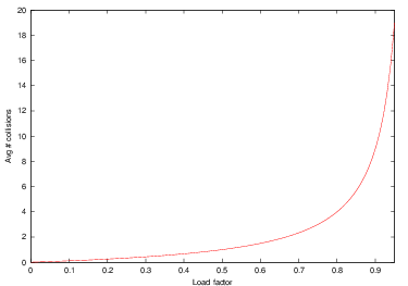
Here you can see the behavior of the function $1/(1-\lambda)$ as the load factor, $\lambda$ increases.
If the table is less than half full ( $\lambda < 0.5$ ), then we are talking about looking at, on average, no more than 2 slots during a search or insert. That’s not bad at all. But as $\lambda$ gets larger, the average number of slots examined grows toward hSize (and, if the table is getting full, then N is approaching hSize, so we are once again degenerating toward O(N) behavior).
So, the rule of thumb for hash tables is to keep them no more than half full. At that load factor, we can treat searches and inserts as $O(1)$ operations. But if we let the load factor get much higher, we start seeing $O(N)$ performance.
Of course, none of the collision resolution schemes we’ve suggested is truly ideal, so keeping the load factor down to a reasonable level is probably even more important in practice than this idealized analysis would indicate.
And quadratic probing does tell us that it is guaranteed to work if the table size is a prime number and if $\lambda < 2$, so if we are going to keep the table no more than half-full anyway, quadratic probing winds up being an attractive choice.
| | 1 of 19
| |