  | 1 of 17


 |   |
| | 1 of 17
| |
The area of graph-processing algorithms is more than large enough to devote an entire course to. In this section we’ll look at just a few of the “classics”, which will, I hope, give you a feel for some of the common patterns shared by most graph processing.
As in our prior lesson, we will be working with the following declarations for most of our graphs:
/*
 * graph.h
 *
 *  Created on: Jul 9, 2020
 *      Author: zeil
 */

#ifndef GRAPH_H_
#define GRAPH_H_

#include <boost/graph/graph_traits.hpp>
#include <boost/graph/adjacency_list.hpp>


typedef boost::adjacency_list<boost::listS, // store edges in lists
		                      boost::vecS, // store vertices in a vector
							  boost::bidirectionalS // a directed graph, with in_edges
							  // no bundled properties on vertices & edges
							  >
                                Graph;
typedef boost::graph_traits<Graph> GraphTraits;
typedef GraphTraits::vertex_descriptor Vertex;
typedef GraphTraits::edge_descriptor Edge;


#endif /* GRAPH_H_ */
Sometimes we need to arrange things according to a partial order: a transitive ordering relation in which for any two elements it is possible that
a<ba=ba>ba is incomparable to bThis last possibility distinguishes partial order operations from the more familiar total order operations, such as < on integers, that are guaranteed to use only the first three of the above four options.
The possibility that some pairs of elements may be incomparable to one another makes sorting via a partial order very different from conventional sorting.
Consider the relation among college courses defined as:
a<b if course a is listed as a prerequisite for ba==b if a and b are the same courseFor example, in the ODU CS dept., we have
cs150<cs250,cs170<cs270,cs150<cs381,cs250<cs361,cs361<cs350,cs250<cs355,cs381<cs355,cs381<cs390,cs270<cs471,cs361<cs471
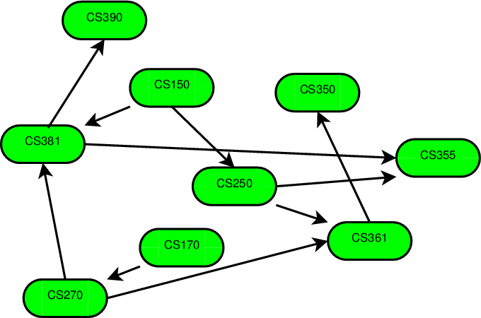
We can represent this as the graph shown here. Each directed edge goes from a prerequisite to a course dependent upon it.
Now, the prerequisite relation holds only between selected pairs of courses. cs150 is not a prerequisite for cs361, but the collection of prerequisites makes it clear that one must take cs150 before taking cs361.
We can define a new relationship “must-be-taken-before” (which I’ll symbolize as “$\prec$”) by starting with the prerequisite relationship, and then insisting that:
\[ a \prec c \; \mbox{if} \; a \prec b \, \wedge \, b \prec c. \]
You may recognize the above rule as a statement that $\prec$ is transitive. This transitive rule adds new, implied, orderings to the “must-be-taken-before” relation. Whenever we have a rule for adding items to a set (based on the items already in there) and we apply it over and over again until we can get no more new items, we call that taking the closure of the rule on that set. So “must-be-taken-before” is called the transitive closure of the prerequisite relation.
We can interpret the transitive closure of a partial order in terms of the graph of that partial order. A pair of vertices v and w are related by \( v <_{\mbox{closed}} w \) in the transitive closure if there is a path from v to w in the graph of the original $<$ relation.
Transitive closures of orderings are often quite useful. For example, the transitive closure of the prerequisite order can be used to determine if a student’s planned sequence for taking CS courses is “legal”. If a student plans to take course a before taking b, this is legal only if !($b \prec_{\mbox{closed}} a$).
As another example, consider the set of formulas that could be entered into a spreadsheet (e.g., Microsoft’s Excel or OpenOffice’s Calc). Spreadsheets store formulas in “cells”. Each cell is identified by its column (using letters) and row (using numbers).
a1 = 10
a2 = 20
a3 = a1 + a2
b1 = 2*a1
b2 = 2*a2
b3 = b1 + b2 + c1
c1 = a3 / a1 / a2
A practical problem faced by all spreadsheet implementors is what order to process the formulas in. If, for example, we evaluate b3 before c1 has been evaluated, we can’t expect to get meaningful results.
Define a partial order as follows:
Let
xandybe any two formulas
x<yif the left-hand side variable ofxappears on the right-hand side ofy
x==yif they are the same formula
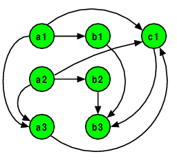
a1 = 10
a2 = 20
a3 = a1 + a2
b1 = 2*a1
b2 = 2*a2
b3 = b1 + b2 + c1
c1 = a3 / a1 / a2
The graph here captures that partial order. Again, the transitive closure of this order is interesting, as it defines a “must-be-evaluated-before” relation.
A topological sort is an ordered list of the vertices in a directed acyclic graph such that, if there is a path from v to w in the graph, then v appears before w in the list.
A topological sort of the course prerequisite graph would be a possible sequence in which a student might take classes. A topological sort of the spreadsheet graph would be an order in which the formulas could be evaluated.
Define the indegree of a vertex as the number of edges pointing to it.
A node of indegree 0 can be placed at the start of the sorted order, since there is clearly nothing that must precede it.
There must be at least one vertex of indegree 0.
If not, the graph has a cycle and no topological sort exists.
Once we have placed all nodes of indegree 0 in the list, we can then add all nodes whose indegree would be zero except for edges from the nodes already placed.
Repeating this process yields a topological sort.
Here is the code for a topological sort.
vector<Vertex> topologicalSort (const Graph& g)
{
	// Step 1: get the indegrees of all vertices. Place vertices with
	// indegree 0 into a queue.
	unsigned nVertices = std::distance(vertices(g).first, vertices(g).second);
	vector<int> inDegree(nVertices);
	vector<Vertex> sorted;

	queue<Vertex, list<Vertex> > q;
	auto allVertices = vertices(g);
	for (auto v = allVertices.first; v != allVertices.second; ++v)
	{
		auto incoming = in_edges(*v, g);
		inDegree[*v] = distance(incoming.first, incoming.second);
		if (inDegree[*v] == 0)
			q.push(*v);
	}

	// Step 2. Take vertices from the q, one at a time, and add to sorted.
	// As we do, pretend that we have deleted these vertices from the graph,
	// decreasing the indegree of all adjacent nodes. If any nodes attain an
	// indegree of 0 because of this, add them to the queue.
	while (!q.empty())
	{
		Vertex v = q.front();
		q.pop();

		sorted.push_back(v);

		auto outEdges = out_edges(v,g);
		for (auto e = outEdges.first; e != outEdges.second; ++e)
		{
			Vertex adjacent = target(*e, g);
			inDegree[adjacent] = inDegree[adjacent] - 1;
			if (inDegree[adjacent] == 0)
				q.push (adjacent);
		}
	}

	// Step 3:  Did we finish the entire graph?
	if (sorted.size() != nVertices)
	{
		sorted.clear();
	}
	return sorted;
}
Let’s consider it a step at a time.
vector<Vertex> topologicalSort (const Graph& g)
{
    // Step 1: get the indegrees of all vertices. Place vertices with
    // indegree 0 into a queue.
    unsigned nVertices = num_vertices(g);
    vector<int> inDegree(nVertices);
    vector<Vertex> sorted;

    queue<Vertex, list<Vertex> > q;
    auto allVertices = vertices(g);
    for (auto v = allVertices.first; v != allVertices.second; ++v)
    {
        auto incoming = in_edges(*v, g);
        inDegree[*v] = in_degree(*v, g);
        if (inDegree[*v] == 0)
            q.push(*v);
    }
In step 1, we get the indegrees of all the vertices, putting them into a map inDegree whose key type is Vertex and whose associated data is unsigned. I’ve chosen to use an vector for this code, but in general we would use a map and you should probably try to think of it as such. Either way, vector or (unordered) map, updating and accessing this data should be O(1).
As we do this, we also add any vertices whose indegree is zero into a queue, q.
// Step 2. Take vertices from the q, one at a time, and add to sorted.
    // As we do, pretend that we have deleted these vertices from the graph,
    // decreasing the indegree of all adjacent nodes. If any nodes attain an
    // indegree of 0 because of this, add them to the queue.
    while (!q.empty())
    {
        Vertex v = q.front();
        q.pop();

        sorted.push_back(v);

        auto outEdges = out_edges(v,g);
        for (auto e = outEdges.first; e != outEdges.second; ++e)
        {
            Vertex adjacent = target(*e, g);
            inDegree[adjacent] = inDegree[adjacent] - 1;
            if (inDegree[adjacent] == 0)
                q.push (adjacent);
        }
    }
In step 2, we repeatedly remove vertices from the queue and add them to the sorted list output, sorted. We can do this because we know that there is nothing in the graph that needs to come before these vertices.
We then look at the outgoing edges of each vertex, and reduce the inDegree values of the neighboring vertices to simulate having removed v from the graph. If doing this causes any of their (simulated) indegrees to become zero, we add them to the queue, because we know that there is nothing remaining in the graph that needs to come before these vertices.
	// Step 3:  Did we finish the entire graph?
	if (sorted.size() != nVertices)
	{
		sorted.clear();
	}
	return sorted;
}
Finally, in step 3, we check to see if all the vertices have been “removed” from the graph and placed into the sorted list. If so, we have successfully found a topological sort. If not, then no topological sort is possible (the graph must have a cycle).
Try out the topological sort in an animation. (This code is slightly different from what we have just gone over, as it predates the Boost graph library, but you should still be able to follow the flow of the algorithm.)
In analyzing this algorithm, we will assume that the graph is implementing using adjacency lists, and that the inDegree map is implemented using a vector-like structure.
vector<Vertex> topologicalSort (const Graph& g)
{
    // Step 1: get the indegrees of all vertices. Place vertices with
    // indegree 0 into a queue.
    unsigned nVertices = num_vertices(g);
    vector<int> inDegree(nVertices);
    vector<Vertex> sorted;

    queue<Vertex, list<Vertex> > q;
    auto allVertices = vertices(g);
    for (auto v = allVertices.first; v != allVertices.second; ++v)
    {
        auto incoming = in_edges(*v, g);          // O(1)
        inDegree[*v] = in_degree(*v, g);          // O(|in_degree(*v,g)|)
        if (inDegree[*v] == 0)                    // O(1)
            q.push(*v);                           // O(1)
    }
In step 1, most of the loop body is $O(1)$. The exception is the in_degree call, which returns the number of edges incoming to v. Because edges are being stored in a std::list, in_degree relies on the std::list::size(), function, which is O(N) where N is the length of the list. In this case, that N is the indegree of the vertex *v.
The loop itself goes around once for every vertex in the graph. So the number of iterations of this loop is $|V|$, the number of vertices.
Now, *v is a different vertex each time around the loop. Hence the in-degree of *v is also going to vary each time arounf the loop. So we cannot use the shortcuto of multiplying the number of iterations by the body complexty. We need to actually sum up
\[ O\left(\sum_{v \in g} in-degree(v)\right) \]
Now, each edge in g contributes to the in-degree of exactly one vertex. So the sum of all of the in-degrees of all the vertices is simply the number of edges in g, generally written as $|E|$.
vector<Vertex> topologicalSort (const Graph& g)
{
    // Step 1: get the indegrees of all vertices. Place vertices with
    // indegree 0 into a queue.
    unsigned nVertices = num_vertices(g);
    vector<int> inDegree(nVertices);
    vector<Vertex> sorted;

    queue<Vertex, list<Vertex> > q;
    auto allVertices = vertices(g);
    for (auto v = allVertices.first; v != allVertices.second; ++v) //cond: O(1) # |V| total: O(|E|)
    {  // body: O(|in_degree(*v,g)|)
        auto incoming = in_edges(*v, g);          // O(1)
        inDegree[*v] = in_degree(*v, g);          // O(|in_degree(*v,g)|)
        if (inDegree[*v] == 0)                    // O(1)
            q.push(*v);                           // O(1)
    }
Looking at the remainder of step 1:
vector<Vertex> topologicalSort (const Graph& g)
{
    // Step 1: get the indegrees of all vertices. Place vertices with
    // indegree 0 into a queue.
    unsigned nVertices = num_vertices(g);
    vector<int> inDegree(nVertices);  // O(|V|)
    vector<Vertex> sorted;            // O(1)

    queue<Vertex, list<Vertex> > q;  // O(1)
    auto allVertices = vertices(g);  // O(1)
    //  O(|E|)
We therefore conclude that the entire step 1 is $O(|V|+|E|)$. ($|E|$ has the potential to be as larges as $|V|^2$, but it is also possible to have vertices with no incoming or outgoing edges, in which case $|V|$ could be larger then $|E|$, so we cannot safely assume that either dominates the other.)
bool topologicalSort (const DiGraph& g, list<Vertex>& sorted)
{
  // O(|V| + |E|)

  // Step 2. Take vertices from the q, one at a time, and add to sorted.
  // As we do, pretend that we have deleted these vertices from the graph,
  // decreasing the indegree of all adjacent nodes. If any nodes attain an
  // indegree of 0 because of this, add them to the queue.
  while (!q.empty())
    {
      Vertex v = q.front();
      q.pop();

      sorted.push_back(v);

      auto outEdges = out_edges(v,g);
      for (auto e = outEdges.first; e != outEdges.second; ++e)
      {
          Vertex adjacent = target(*e, g);
          inDegree[adjacent] = inDegree[adjacent] - 1;
          if (inDegree[adjacent] == 0)
            q.push (adjacent);
      }
    }
    ⋮
Looking at the inner loop of step 2, we see that everything in the body is O(1).
bool topologicalSort (const DiGraph& g, list<Vertex>& sorted)
{
  O(|V| + |E|)

  // Step 2. Take vertices from the q, one at a time, and add to sorted.
  // As we do, pretend that we have deleted these vertices from the graph,
  // decreasing the indegree of all adjacent nodes. If any nodes attain an
  // indegree of 0 because of this, add them to the queue.
  while (!q.empty())
    {
      Vertex v = q.front();
      q.pop();

      sorted.push_back(v);

      auto outEdges = out_edges(v,g);
      for (auto e = outEdges.first; e != outEdges.second; ++e)
      {
          Vertex adjacent = target(*e, g);               // O(1)
          inDegree[adjacent] = inDegree[adjacent] - 1;   // O(1)
          if (inDegree[adjacent] == 0)                   // cond: O(1) total: O(1)
            q.push (adjacent);                           // O(1)
      }
    }
    ⋮
And the simple statements in the outer loop (everything except for the inner loop) are O(1).
bool topologicalSort (const DiGraph& g, list<Vertex>& sorted)
{
  O(|V| + |E|)

  // Step 2. Take vertices from the q, one at a time, and add to sorted.
  // As we do, pretend that we have deleted these vertices from the graph,
  // decreasing the indegree of all adjacent nodes. If any nodes attain an
  // indegree of 0 because of this, add them to the queue.
  while (!q.empty())
    {
      Vertex v = q.front();                              // O(1)
      q.pop();                                           // O(1)

      sorted.push_back(v);                               //O(1) [amortized]

      auto outEdges = out_edges(v,g);
      for (auto e = outEdges.first; e != outEdges.second; ++e) /// cond: O(1) iter: O(1)
      {
          Vertex adjacent = target(*e, g);               // O(1)
          inDegree[adjacent] = inDegree[adjacent] - 1;   // O(1)
          if (inDegree[adjacent] == 0)                   // cond: O(1) total: O(1)
            q.push (adjacent);                           // O(1)
      }
    }
    ⋮
Now, at this point our normal copy-and-paste approach breaks down. The number of iterations of the inner loop may be different for each vertex visited by the outer loop.
But, let’s just stop and think about what’s going on here.
So the statements in the body of the inner loop get executed $|E|$ times; the other statements in the outer loop get visited $|V|$ times. Since all of these statements are $O(1)$, the total cost is $O(|V|+|E|)$.
bool topologicalSort (const DiGraph& g, list<Vertex>& sorted)
{
    O(|V| + |E|)
    O(|V| + |E|)

	// Step 3:  Did we finish the entire graph?
	if (sorted.size() != nVertices)   // O(1)
	{
		sorted.clear();               // O(|V|)
	}
	return sorted;                    // O(1)
}
In step 3, the only non-trivial operations is clearing the sorted list (done when we can’t find a solution). Since this list is actually a list of vertices that we have successfully sorted, it contains at most $|V|$ elements, and so the clear operation is $O(|V|)$.
That makes the worst case for the step 3 “if” statement $O(|V|)$ as well.
bool topologicalSort (const DiGraph& g, list<Vertex>& sorted)
{
  O(|V| + |E|)
  O(|V| + |E|)
  O(|V|)
}
So the total cost of the topological sort is $O(|V| + |E|)$.
(Note: this does not mean that topological sorts are faster than conventional sorts — the number of edges can be as high as $|V|^{\mbox{2}}$, so this is actually more comparable to the slowest of our conventional sorting algorithms. That’s the penalty we pay for working with partial orders.
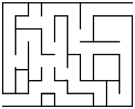
Example: Given a maze, find the shortest path from the start to the finish.
To see how this relates to graphs, try numbering each intersection and dead-end in the graph.

Now we can form a graph by assigning a vertex to each numbered location, and connecting two vertices with an edge if it is possible to go directly from one vertex’s position to the other without passing through another numbered position.
This graph captures the notion of “adjacent” numbered locations.
And the problem of finding the shortest path through the maze has now been reduced to (changed into) the problem of finding the shortest path between the starting and ending vertex of the graph.
Now, there’s lots of ways to find a path through a maze. There’s the venerable “keep your right hand on the wall” technique.
This would take us through positions 1, 2, 3, 2, 4, 9, 10, 12, 10, 11, 10, 9, 13, 14, 13, …
This technique often finds a path, but not necessarily the shortest.
And it’s only guaranteed to find a path if the graph (maze) is acyclic (or if, as is the case here, both the entrance and exit are on the outer edge of the maze).
A variant is the “keep your right hand on the wall and trail a string behind you” technique (first recorded in the old Greek tale of Theseus and the Minotaur in the great labyrinth of Crete).
This avoids problems with cycles, because if you ever come across your own string, you turn around and start back, rewinding the string until you come to a place where you can make a new right turn.
Still may not find the shortest path
A better solution is based on the following idea:
You may recognize this as essentially our breadth-first traversal algorithm, with just a few changes:
Now let’s render this idea into code.
Here is the entire algorithm.
vector<Vertex> findShortestPath (
        const Graph& g,
        Vertex start,
        Vertex finish)
{
    unsigned nVertices = num_vertices(g);
    vector<Vertex> cameFrom (nVertices);
    vector<Vertex> path;

    vector<unsigned> dist (nVertices, nVertices);
    dist[start] = 0;

    queue<Vertex, list<Vertex> > q;
    q.push (start);

    // From each vertex in queue, update distances of adjacent vertices
    while (!q.empty() && (dist[finish] == nVertices))
    {
        Vertex v = q.front();
        unsigned d = dist[v];
        q.pop();
        auto outGoing = out_edges(v, g);
        for (auto e = outGoing.first; e != outGoing.second; ++e)
        {
            Vertex w = target(*e, g);
            if (dist[w] > d + 1)
            {
                dist[w] = d + 1;
                q.push (w);
                cameFrom[w] = v;
            }
        }
    }
    // Extract path
    if (dist[finish] != nVertices)
    {
        Vertex v = finish;
        while (!(v == start))
        {
            path.push_back(v);
            v = cameFrom[v];
        }
        path.push_back(start);
    }
    reverse (path.begin(), path.end());

    return path;
}
Again, let’s take it apart, one piece at a time.
vector<Vertex> findShortestPath (
        const Graph& g,
        Vertex start,
        Vertex finish)
{
    unsigned nVertices = num_vertices(g);
    vector<Vertex> cameFrom (nVertices);
    vector<Vertex> path;

    vector<unsigned> dist (nVertices, nVertices);  ➀
    dist[start] = 0;

    queue<Vertex, list<Vertex> > q;
    q.push (start);
We will use two data structures to keep track of information about the vertices in our graph:
dist[v] is the smallest number of steps in which we believe a vertex v can be reached when starting from start.
This is initialized at ➀ to hold values larger than any possible “real” distance, namely, nVertices. (The longest possible real path, if the vertices formed a straight line, would be nVertices-1).
cameFrom[v] will hold the vertex that we used to reach v on the shortest path that we were able to find.
In addition to these “maps”, we will use path to hold our final output, and a queue q to manage the breadth-first travesal. q is initialized to hold the start vertex.
The first loop simply assigns to each vertex a distance value that is larger than any legitimate path could be. The exception is that the start vertex is given a distance of 0.
Then we create a queue, placing the start vertex into it.
    // From each vertex in queue, update distances of adjacent vertices
    while (!q.empty() && (dist[finish] == nVertices))
    {
        Vertex v = q.front();
        unsigned d = dist[v];
        q.pop();
        auto outGoing = out_edges(v, g);
        for (auto e = outGoing.first; e != outGoing.second; ++e)
        {
            Vertex w = target(*e, g);
            if (dist[w] > d + 1)
            {
                dist[w] = d + 1;
                q.push (w);
                cameFrom[w] = v;
            }
        }
    }
The main loop removes vertices, one at a time, from the queue. The shortest known distance to that node is computed in d. Then each adjacent vertex is examined. If its best-known distance (so far) from start is bigger than d+1, we now know that we can get there “faster” because the distance to the current vertex is d, and this adjacent vertex is only one step away from that. So we set its distance to d+1 and place it on the queue, so that eventually we will examine all the vertices one step away from it.
We keep this up until we have computed a new, shortest distance for the finish vertex or until the queue is empty (in which case we conclude that there’s no way to get from the start vertex to the finish).
    // Extract path
    if (dist[finish] != nVertices)
    {
        Vertex v = finish;
        while (!(v == start))
        {
            path.push_back(v);
            v = cameFrom[v];
        }
        path.push_back(start);
    }
    reverse (path.begin(), path.end());

    return path;
}
The final loop traces back from the finish by using the information we recorded about how we first reached each vertex.
However, since we are starting from the finish and working our way back to the start, this loop actually builds our shortest path backwards. The std::reverse function reverses that ordering to put the path into the desiredt start to finish order.
Again, I will assume an adjacency list implementation of the graph. With this in mind, let’s just start by labeling everything that is obviously $O(1)$.
vector<Vertex> findShortestPath (
        const Graph& g,
        Vertex start,
        Vertex finish)
{
    unsigned nVertices = num_vertices(g);  // O(1)
    vector<Vertex> cameFrom (nVertices);   // O(1)
    vector<Vertex> path;                   // O(1)

    vector<unsigned> dist (nVertices, nVertices);
    dist[start] = 0;                       // O(1)

    queue<Vertex, list<Vertex> > q;        // O(1)
    q.push (start);                        // O(1)

    // From each vertex in queue, update distances of adjacent vertices
    while (!q.empty() && (dist[finish] == nVertices)) // cond: O(1)
    {
        Vertex v = q.front();               // O(1)
        unsigned d = dist[v];               // O(1)
        q.pop();                            // O(1)
        auto outGoing = out_edges(v, g);    // O(1)
        for (auto e = outGoing.first; e != outGoing.second; ++e)
        {
            Vertex w = target(*e, g);       // O(1)
            if (dist[w] > d + 1)            // cond: O(1)
            {
                dist[w] = d + 1;            // O(1)
                q.push (w);                 // O(1)
                cameFrom[w] = v;            // O(1)
            }
        }
    }
    // Extract path
    if (dist[finish] != nVertices)         // cond: O(1)
    {
        Vertex v = finish;                 // O(1)
        while (!(v == start))              // cond: O(1)
        {
            path.push_back(v);             // O(1) [amortized]
            v = cameFrom[v];               // O(1)
        }
        path.push_back(start);            // O(1) [amortized]
    }
    reverse (path.begin(), path.end());

    return path;                         // O(1)
}
Looking at the initialization code, the declaration of dist initializes all nVertices elements of the vector with the value nVertices. That makes it O(nVertices) or, more compactly, $O(|V|)$.
    unsigned nVertices = num_vertices(g);  // O(1)
    vector<Vertex> cameFrom (nVertices);   // O(1)
    vector<Vertex> path;                   // O(1)

    vector<unsigned> dist (nVertices, nVertices);  // O(|V|)
    dist[start] = 0;                       // O(1)

    queue<Vertex, list<Vertex> > q;        // O(1)
    q.push (start);                        // O(1)
That entire block of code is therefore $O(|V|)$.
Turning our attention to the inner (for) loop body, we can see that the if statement inside is $O(1)$.
vector<Vertex> findShortestPath (
        const Graph& g,
        Vertex start,
        Vertex finish)
{
    // O(|V|)

    // From each vertex in queue, update distances of adjacent vertices
    while (!q.empty() && (dist[finish] == nVertices)) // cond: O(1)
    {
        Vertex v = q.front();               // O(1)
        unsigned d = dist[v];               // O(1)
        q.pop();                            // O(1)
        auto outGoing = out_edges(v, g);    // O(1)
        for (auto e = outGoing.first; e != outGoing.second; ++e)
        {
            Vertex w = target(*e, g);       // O(1)
            if (dist[w] > d + 1)            // cond: O(1) total: O(1)
            {
                dist[w] = d + 1;            // O(1)
                q.push (w);                 // O(1)
                cameFrom[w] = v;            // O(1)
            }
        }
    }
    // Extract path
    if (dist[finish] != nVertices)         // cond: O(1)
    {
        Vertex v = finish;                 // O(1)
        while (!(v == start))              // cond: O(1)
        {
            path.push_back(v);             // O(1) [amortized]
            v = cameFrom[v];               // O(1)
        }
        path.push_back(start);            // O(1) [amortized]
    }
    reverse (path.begin(), path.end());

    return path;                         // O(1)
}
And that means that the entire inner loop body is $O(1)$.
vector<Vertex> findShortestPath (
        const Graph& g,
        Vertex start,
        Vertex finish)
{
    // O(|V|)

    // From each vertex in queue, update distances of adjacent vertices
    while (!q.empty() && (dist[finish] == nVertices)) // cond: O(1)
    {
        Vertex v = q.front();               // O(1)
        unsigned d = dist[v];               // O(1)
        q.pop();                            // O(1)
        auto outGoing = out_edges(v, g);    // O(1)
        for (auto e = outGoing.first; e != outGoing.second; ++e)
        {
		  // O(1)
        }
    }
    // Extract path
    if (dist[finish] != nVertices)         // cond: O(1)
    {
        Vertex v = finish;                 // O(1)
        while (!(v == start))              // cond: O(1)
        {
            path.push_back(v);             // O(1) [amortized]
            v = cameFrom[v];               // O(1)
        }
        path.push_back(start);            // O(1) [amortized]
    }
    reverse (path.begin(), path.end());

    return path;                         // O(1)
}
Now, looking at that inner loop, we see that it iterates over the outgoing edges of a vertex. Since the outer loop goes through all of the vertices, the total number of executions of the inner loop body, summed over all the iterations of the outer loop, will be $|E|$.
vector<Vertex> findShortestPath (
        const Graph& g,
        Vertex start,
        Vertex finish)
{
    // O(|V|)

    // From each vertex in queue, update distances of adjacent vertices
    // O(|E|)  [inner loop total]
    while (!q.empty() && (dist[finish] == nVertices)) // cond: O(1)
    {
        Vertex v = q.front();               // O(1)
        unsigned d = dist[v];               // O(1)
        q.pop();                            // O(1)
        auto outGoing = out_edges(v, g);    // O(1)
          ⋮
    }
    // Extract path
    if (dist[finish] != nVertices)         // cond: O(1)
    {
        Vertex v = finish;                 // O(1)
        while (!(v == start))              // cond: O(1)
        {
            path.push_back(v);             // O(1) [amortized]
            v = cameFrom[v];               // O(1)
        }
        path.push_back(start);            // O(1) [amortized]
    }
    reverse (path.begin(), path.end());

    return path;                         // O(1)
}
The remaining portions of the outer loop do only $O(1)$ for each iteration, and there are |V| iterations.
vector<Vertex> findShortestPath (
        const Graph& g,
        Vertex start,
        Vertex finish)
{
    // O(|V|)

    // From each vertex in queue, update distances of adjacent vertices
    // O(|E|)  [inner loop total]
    while (!q.empty() && (dist[finish] == nVertices)) // cond: O(1) #: |V|  total O(|V|)
    {  // body: O(1)
        Vertex v = q.front();               // O(1)
        unsigned d = dist[v];               // O(1)
        q.pop();                            // O(1)
        auto outGoing = out_edges(v, g);    // O(1)
          ⋮
    }
    // Extract path
    if (dist[finish] != nVertices)         // cond: O(1)
    {
        Vertex v = finish;                 // O(1)
        while (!(v == start))              // cond: O(1)
        {
            path.push_back(v);             // O(1) [amortized]
            v = cameFrom[v];               // O(1)
        }
        path.push_back(start);            // O(1) [amortized]
    }
    reverse (path.begin(), path.end());

    return path;                         // O(1)
}
And we can now reduce the middle part of the algorithm:
vector<Vertex> findShortestPath (
        const Graph& g,
        Vertex start,
        Vertex finish)
{
    // O(|V|)

    // From each vertex in queue, update distances of adjacent vertices
    // O(|E|)
    // O(|V|)

    // Extract path
    if (dist[finish] != nVertices)         // cond: O(1)
    {
        Vertex v = finish;                 // O(1)
        while (!(v == start))              // cond: O(1)
        {
            path.push_back(v);             // O(1) [amortized]
            v = cameFrom[v];               // O(1)
        }
        path.push_back(start);            // O(1) [amortized]
    }
    reverse (path.begin(), path.end());

    return path;                         // O(1)
}
In the final section of the algorithm, the while loop executes once for each vertex along the shortest path that we found from start to finish. In the worst case, the vertices form a straight line from start to finish, and the loop executes $|V|-1$ times.
vector<Vertex> findShortestPath (
        const Graph& g,
        Vertex start,
        Vertex finish)
{
    // O(|V|)

    // O(|E|)
    // O(|V|)

    // Extract path
    if (dist[finish] != nVertices)         // cond: O(1)
    {
        Vertex v = finish;                 // O(1)
        while (!(v == start))              // cond: O(1) #: |V|-1 total: O(|V|)
        {
            path.push_back(v);             // O(1) [amortized]
            v = cameFrom[v];               // O(1)
        }
        path.push_back(start);            // O(1) [amortized]
    }
    reverse (path.begin(), path.end());

    return path;                         // O(1)
}
That makes the then-part of the if $O(|V|)$, so the entire if statement is O(|V|).
vector<Vertex> findShortestPath (
        const Graph& g,
        Vertex start,
        Vertex finish)
{
    // O(|V|)

    // O(|E|)
    // O(|V|)

    // O(|V|)
    reverse (path.begin(), path.end());

    return path;                         // O(1)
}
The reverse function runs in linear time, proportional to the number of elements it is given. We have already said that the number of elements in path will be bounded by |V|.
vector<Vertex> findShortestPath (
        const Graph& g,
        Vertex start,
        Vertex finish)
{
    // O(|V|)

    // O(|E|)
    // O(|V|)

    // O(|V|)
    reverse (path.begin(), path.end());  // O(|V|)

    return path;                         // O(1)
}
Finally, we just add everything up and conclude that this function overall is $O(|V| + |E|)$.
Now, let’s consider a more general form of the same problem. Attach to each edge a weight indicating the cost of traversing that edge.
Find a path between designated start and finish nodes that minimizes the sum of the weights of the edges in the path.

Example: finding the cheapest airline route:
What’s the cheapest way to get from D.C. to N.Y?
To deal with this problem, we adapt the unweighted shortest path algorithm.
The algorithm was:
Keep nodes in a collection (queue).
From the collection, we extract a node closest to the start.
From that node we considered the smallest possible step (always 1), updating the distances of the adjacent nodes accordingly.
With weighted graphs, we do the same, but the step size is determined by the weights. We use a priority queue to keep track of the nodes closest to the start.
We will use a map to associate with each vertex the shortest distance (cost, in the airline example) known so far from the start to that vertex. This value starts impossibly high, so that any path we find to that vertex will look good by comparison.
This algorithm is popularly called Dijkstra’s algorithm, named for its inventor.
/**
 * Find a path through graph g from start to finish that has the smallest
 * possible sum of edge weight.
 *
 * @param g the graph
 * @param start the beginning of the path
 * @param finish the end of the path
 * @param weight a map associating an integer weight with each edge in g
 * @return the minimum-total-cost path from start to finish, or an empty
 *         vector if no path from start to finish exists.
 */
template <typename Graph, typename WeightMap>
std::vector<Vertex> findWeightedShortestPath (
        const Graph& g,
        Vertex start,
        Vertex finish,
        const WeightMap& weight)
{
    // Initialize the distance map and the priority queue
    unsigned nVertices = num_vertices(g);

    std::vector<Vertex> cameFrom (nVertices);

    std::vector<unsigned> dist(nVertices, INT_MAX);
    dist[(int)start] = 0;

    typedef std::pair<int, Vertex> Element;
    std::priority_queue<Element, std::vector<Element>, std::greater<Element> >
    pq;
    pq.push (Element(0, start));

    // Find the shortest path
    while (!pq.empty())
    {
        Element top = pq.top();
        pq.pop();
        Vertex v = top.second;
        if (v == finish) break; // exit when we reach the finish vertex
        int d = dist[v];
        if (top.first == d)
        {
            auto outgoing = out_edges(v, g);
            for (auto e = outgoing.first; e != outgoing.second; ++e)
            {
                Vertex w = target(*e, g);
                unsigned wdist = d+weight.at(*e);
                if (dist[w] > wdist)
                {
                    dist[w] = wDist;
                    pq.push(Element(wDist, w));
                    cameFrom[w] = v;
                }
            }
        }
    }

    // Extract path
    std::vector<Vertex> path;
    Vertex v = finish;
    if (dist[v] != INT_MAX)
    {
        while (!(v == start))
        {
            path.push_back(v);
            v = cameFrom[v];
        }
        path.push_back(start);
    }
    std::reverse(path.begin(), path.end());
    return path;
}
There are really only a few changes from our unweighted min path search.
We replace the queue of Vertices with a priority queue.
The elements of this priority queue are pairs containing a distance and a Vertex. When two std::pair elements are compared with operator<, the first members are compared first. The second members are compared only if the two first members are equal. So the ordering in our priority queue will be determined by the distance component.
As we process each vertex v, we add its shortest-known distance so far to the weight/distance from v to each adjacent vertex w. If that distance is smaller then the shortest-known distance to reach w so far (stored in dist[w]), then we know that we have found a new, shorter, way to get to w and we add an element describing that new distance to w into the priority queue.
It is entirely possible that w will already be in the priority queue, but if so, it will be in there with a larger distance. Because our priority queue, unlike an ordinary queue, always shows the smallest-distance element at the top, this new, shorter distance for w will get processed before any larger values already in the priority queue.
To see how this works, let’s do a walkthrough (desk check) of the algorithm, asking it to find the cheapest route from WashDC to NY.
start: WashDC
finish: NY
pq: <0, WashDC>
cameFrom: ??
dist: {(Boston, 9999999), (Norfolk, 9999999), (NY, 9999999),
       (Raleigh, 9999999), (WashDC, 0)}
When we finish the initialization, all cities will have been assigned a dist of INT_MAX, which I denote in this walkthrough as 9999999.
We enter the outer loop, and pop the top element from the priority queue.
start: WashDC
finish: NY
pq:
cameFrom: ??
dist: {(Boston, 9999999), (Norfolk, 9999999), (NY, 9999999),
       (Raleigh, 9999999), (WashDC, 0)}
v: WashDC
d: 0
d is initialized from dist[v], and we enter the outer loop.
WashDC has three outgoing edges. For the sake of the example, we will assume that edges are processed in alphabetic order of the destination name.
So we start with the WashDC to Boston flight.
start: WashDC
finish: NY
pq:
cameFrom: ??
dist: {(Boston, 9999999), (Norfolk, 9999999), (NY, 9999999),
       (Raleigh, 9999999), (WashDC, 0)}
v: WashDC
d: 0
w: Boston
wDist: 7900
The new shortest (cheapest) path to Boston is computed as d+7900 (the cost of the WashDC to Boston flight being $79.00). This is smaller than the current value in dist[Boston].
start: WashDC
finish: NY
pq: {(7900, Boston)}
cameFrom: {(Boston, WashDC)}
dist: {(Boston, 7900), (Norfolk, 9999999), (NY, 9999999),
       (Raleigh, 9999999), (WashDC, 0)}
v: WashDC
d: 0
w: Boston
wDist: 7900
So we add (wDist, Boston) to the queue, record the new cheaper cost to get to Boston in dist[Boston], and note that in reaching Boston, we came from WashDC.
Then we go back to the start of the inner loop, and consider the flight from WashDC to Norfolk.
start: WashDC
finish: NY
pq: {(5800, Norfolk), (7900, Boston)}
cameFrom: {(Boston, WashDC), (Norfolk, WashDC)}
dist: {(Boston, 7900), (Norfolk, 5800), (NY, 9999999),
       (Raleigh, 9999999), (WashDC, 0)}
v: WashDC
d: 0
w: Norfolk
wDist: 5800
The cost to get to Norfolk via WashDC is computed as 0+6400. That’s cheaper than the value in dist[Norfolk], so we add (wDist, Norfolk) to the queue, record the new cheaper cost to get to Norfolk in dist[Norfolk], and note that in reaching Norfolk, we came from WashDC.
Then we go back to the start of the inner loop, and consider the flight from WashDC to NY.
start: WashDC
finish: NY
pq: {(5800, Norfolk), (7900, Boston), (23900, NY)}
cameFrom: {(Boston, WashDC), (Norfolk, WashDC), (NY, WashDC)}
dist: {(Boston, 7900), (Norfolk, 5800), (NY, 23900),
       (Raleigh, 9999999), (WashDC, 0)}
v: WashDC
d: 0
w: NY
wDist: 23900
The cost to get to NY via WashDC is computed as 0+23900. That’s cheaper than the value in dist[NY], so we add (wDist, NY) to the queue, record the new cheaper cost to get to NY in dist[NY], and note that in reaching NY, we came from WashDC.
That completes the inner loop of outgoing edges from WashDC. So now we move back around the outer loop.
The smallest element in the priority queue is (6400, Norfolk), so we will look at Norfolk next.
start: WashDC
finish: NY
pq: {(7900, Boston), (23900, NY)}
cameFrom: {(Boston, WashDC), (Norfolk, WashDC), (NY, WashDC)}
dist: {(Boston, 7900), (Norfolk, 5800), (NY, 23900),
       (Raleigh, 9999999), (WashDC, 0)}
v: Norfolk
d: 5800
w:
wDist:
The distance value d from the priority queue and from dist[Norfolk] is 5800, so that is our new base distance d for our distance calculation.
Norfolk only has one outgoing edge, so we enter the inner loop and look at hte Norfolk to Raleigh flight.
start: WashDC
finish: NY
pq: {(7900, Boston), (12200, Raleigh), (23900, NY)}
cameFrom: {(Boston, WashDC), (Norfolk, WashDC), (NY, WashDC), (Raleigh, Norfolk)}
dist: {(Boston, 7900), (Norfolk, 5800), (NY, 23900),
       (Raleigh, 12200), (WashDC, 0)}
v: Norfolk
d: 5800
w: Raleigh
wDist: 12200
The cost to get to Raleigh via Norfolk is computed as wDist=d+6400=12200. That’s cheaper than the value in dist[Raleigh], so we add (wDist, Raleigh) to the queue, record the new cheaper cost to get to Raleigh in dist[Raleigh], and note that in reaching Raleigh, we came from Norfolk.
That completes the inner loop of outgoing edges from WashDC. So now we move back around the outer loop.
The smallest element in the priority queue is (7900, Boston), so we will look at Boston next.
start: WashDC
finish: NY
pq: {(12200, Raleigh), (23900, NY)}
cameFrom: {(Boston, WashDC), (Norfolk, WashDC), (NY, WashDC), (Raleigh, Norfolk)}
dist: {(Boston, 7900), (Norfolk, 5800), (NY, 23900),
       (Raleigh, 12200), (WashDC, 0)}
v: Boston
d: 7900
w:
wDist:
The distance value d from the priority queue and from dist[Boston] is 7900, so that is our new base distance d for our distance calculation.
Boston has two outgoing edges, so we enter the inner loop and look at the Boston to NY flight.
start: WashDC
finish: NY
pq: {(12200, Raleigh), (23800, NY), (23900, NY)}
cameFrom: {(Boston, WashDC), (Norfolk, WashDC), (NY, Boston), (Raleigh, Norfolk)}
dist: {(Boston, 7900), (Norfolk, 5800), (NY, 23800),
       (Raleigh, 12200), (WashDC, 0)}
v: Boston
d: 7900
w: NY
wDist:
The cost to get to NY via Boston is computed as wDist=d+15900=23800. That’s cheaper than the value in dist[NY], so we add (wDist, NY) to the queue, record the new cheaper cost to get to NY in dist[NY], and note that in reaching NY, we came from Boston.
Next, we consider the flight from Boston to WashDC.
start: WashDC
finish: NY
pq: {(12200, Raleigh), (23800, NY), (23900, NY)}
cameFrom: {(Boston, WashDC), (Norfolk, WashDC), (NY, Boston), (Raleigh, Norfolk)}
dist: {(Boston, 7900), (Norfolk, 5800), (NY, 23800),
       (Raleigh, 12200), (WashDC, 0)}
v: Boston
d: 7900
w: WashDC
wDist: 15400
The cost to get to WashDC via Boston is computed as wDist=d+7500=15400. That’s more expensive than the value in dist[Wash], so we don’t update anything based on this flight.
That takes care of all of the flights out of Boston, so we are ready to go back to the start of the outer loop. The smallest element in the priority queue is (12200, Raleigh), so we look at Raleigh next.
start: WashDC
finish: NY
pq: {(23800, NY), (23900, NY)}
cameFrom: {(Boston, WashDC), (Norfolk, WashDC), (NY, Boston), (Raleigh, Norfolk)}
dist: {(Boston, 7900), (Norfolk, 5800), (NY, 23800),
       (Raleigh, 12200), (WashDC, 0)}
v: Raleigh
d: 12200
w:
wDist:
The distance 12200 from the priority queue matches dist[Raleigh], so we proceed to look at the outgoing edges from Raleigh. There is only one, the flight from Raleigh to NY.
start: WashDC
finish: NY
pq: {(22300, NY), (23800, NY), (23900, NY)}
cameFrom: {(Boston, WashDC), (Norfolk, WashDC), (NY, Raleigh), (Raleigh, Norfolk)}
dist: {(Boston, 7900), (Norfolk, 5800), (NY, Raleigh),
       (Raleigh, 12200), (WashDC, 0)}
v: Raleigh
d: 12200
w: NY
wDist: 22300
The cost to get to NY via Raleigh is computed as wDist=d+10100=22300. That’s cheaper than the value in dist[NY], so we add (wDist, NY) to the queue, record the new cheaper cost to get to NY in dist[NY], and note that in reaching NY, we came from Raleigh.
We’ve finished all of the outgoing edges from Raleigh, so we are ready to return to the top of the outer loop. The smallest element in the priority queue is (22300, NY).
start: WashDC
finish: NY
pq: {(23800, NY), (23900, NY)}
cameFrom: {(Boston, WashDC), (Norfolk, WashDC), (NY, Raleigh), (Raleigh, Norfolk)}
dist: {(Boston, 7900), (Norfolk, 5800), (NY, Raleigh),
       (Raleigh, 12200), (WashDC, 0)}
v: NY
d: 22300
w:
wDist:
But NY is our finish vertex, so we then break out of the outer loop and drop down to the final step, extracting the path.
start: WashDC
finish: NY
pq: {(23800, NY), (23900, NY)}
cameFrom: {(Boston, WashDC), (Norfolk, WashDC), (NY, Raleigh), (Raleigh, Norfolk)}
dist: {(Boston, 7900), (Norfolk, 5800), (NY, Raleigh),
       (Raleigh, 12200), (WashDC, 0)}
v: NY
path: [ ]
We start v at our finish vertex and create an empty path. Then we enter the final loop.
start: WashDC
finish: NY
pq: {(23800, NY), (23900, NY)}
cameFrom: {(Boston, WashDC), (Norfolk, WashDC), (NY, Raleigh), (Raleigh, Norfolk)}
dist: {(Boston, 7900), (Norfolk, 5800), (NY, Raleigh),
       (Raleigh, 12200), (WashDC, 0)}
v: Raleigh
path: [NY]
We push v (NY) onto the back of the path and set v to cameFrom[NY].
start: WashDC
finish: NY
pq: {(23800, NY), (23900, NY)}
cameFrom: {(Boston, WashDC), (Norfolk, WashDC), (NY, Raleigh), (Raleigh, Norfolk)}
dist: {(Boston, 7900), (Norfolk, 5800), (NY, Raleigh),
       (Raleigh, 12200), (WashDC, 0)}
v: Norfolk
path: [NY, Raleigh]
We push v (Raleigh) onto the back of the path and set v to cameFrom[Raleigh].
start: WashDC
finish: NY
pq: {(23800, NY), (23900, NY)}
cameFrom: {(Boston, WashDC), (Norfolk, WashDC), (NY, Raleigh), (Raleigh, Norfolk)}
dist: {(Boston, 7900), (Norfolk, 5800), (NY, Raleigh),
       (Raleigh, 12200), (WashDC, 0)}
v: WashDC
path: [NY, Raleigh, Norfolk]
We push v (Norfolk) onto the back of the path and set v to cameFrom[Norfolk].
start: WashDC
finish: NY
pq: {(23800, NY), (23900, NY)}
cameFrom: {(Boston, WashDC), (Norfolk, WashDC), (NY, Raleigh), (Raleigh, Norfolk)}
dist: {(Boston, 7900), (Norfolk, 5800), (NY, Raleigh),
       (Raleigh, 12200), (WashDC, 0)}
v: WashDC
path: [NY, Raleigh, Norfolk, WashDC]
v is now equal to start, so we exit the loop.
We push start (WashDC) onto the back of the path.
start: WashDC
finish: NY
pq: {(23800, NY), (23900, NY)}
cameFrom: {(Boston, WashDC), (Norfolk, WashDC), (NY, Raleigh), (Raleigh, Norfolk)}
dist: {(Boston, 7900), (Norfolk, 5800), (NY, Raleigh),
       (Raleigh, 12200), (WashDC, 0)}
v: WashDC
path: [WashDC, Norfolk, Raleigh, NY]
We reverse the path, and we are done.
The cheapest way to get from WashDC is to fly through Norfolk and then Raleigh.
  | 1 of 20 |   |
Try out the a similar coding of Dijkstra’s algorithm in an animation.
Structurally, Dijkstra’s algorithm is similar to the unweighted shortest path algorithm, so we might expect that the analysis will also be similar.
We know that in the main section of the unweighted astatements in the inner loop are executed at most $|E|$ times and the remaining statements in the outer loop are executed at most $|V|$ times.
In the weighted algorithm, the outer loop could repeat as many as $|E|$ times but, still, no edge is ever processed more than once. So not statement in the inner or outer loops will be executed more than $|E|$ times.
In Dikstra’s algorithm, the outer loop pops from a priority queue. The inner loop pushes elements into a priority queue. We know that these operations take time proportional to the log of the size of the priority queue.
In the worst case, every edge contributes one element to the priority queue. So we can use $|E|$ as the bound of the priority queue size, and argue that the algorithm would be dominated by the $O(|E| \log |E|)$ time to push and pop $|E|$ elements on the priority queue.
This can be simplified slightly if we are not using a multi-graph. Then $|E| \leq |V|^2$, so we can write $O(|E| \log |E|) = O(|E| \log (|V|^2))$. But in general $\log x^2 = 2 \log x$, so $O(|E| \log (|V|^2))* simplifies to $O(2 |E| \log |V|)$ and then simplifies further to $O(|E| \log |V|)$.
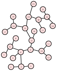
Consider the problem of hooking up a number of phone outlets in various locations throughout a building.
Given the blueprints, we can determine the amount of wire required to connect any two phone jacks.
We want to connect every jack, using a minimum amount of wire.
Form a graph with
a vertex for each phone jack
undirected edges labeled by the wiring distance
This is not a minimum path problem, because the phone outlets don’t need to be connected in a straight line – they just need to be connected somehow.
We want to find the subgraph of the original graph that
is connected
spans (i.e., has every vertex and some edges from) the original graph
Involves the edges leading the minimum possible sum of weights
A little thought will show that for any solution to this problem, there will only be one path from any vertex to any other vertex (if there were more than one, we would have a redundant connection somewhere). Any connected graph with that property is a tree, so this problem is known as the “minimum spanning tree” problem.
One solution, Prim’s algorithm, turns out to be almost identical to Dijkstra’s. The main difference is that, instead of keeping track of the total distance to each vertex from the start, we base our priority queue on the minimum distance to the vertex from any vertex that has already been processed.
/**
 * Find a minimum spanning tree within g rooted at start.
 *
 * @param g the graph
 * @param weight a map associating an integer weight with each edge in g
 * @return a set of edges comprising a minimum spanning tree.
 */
template <typename Graph, typename WeightMap>
std::unordered_set<Edge, boost::hash<Edge>> findMinSpanTree (
   const Graph& g,
   const WeightMap& weight)
{      // Prim's Algorithm
	// Initialize the distance map and the priority queue
	auto allVertices = vertices(g);
	unsigned nVertices = num_vertices(g);

	std::vector<Edge> cameFrom(nVertices);
    std::vector<unsigned> dist(nVertices, INT_MAX);
	dist[*(allVertices.first)] = 0;

	typedef std::pair<int, Vertex> Element;
	std::priority_queue<Element, std::vector<Element>, std::greater<Element> >
	pq;
	pq.push (Element(0, *(allVertices.first)));

	// Find the shortest path
	while (!pq.empty())
	{
		Element top = pq.top();
		pq.pop();
		Vertex v = top.second;
		int d = dist[v];
		if (top.first == d)
		{
			auto outgoing = out_edges(v, g);
			for (auto e = outgoing.first; e != outgoing.second; ++e)
			{
				Vertex w = target(*e, g);
				if (dist[w] > weight.at(*e))
				{
					unsigned newDist = weight.at(*e);
					dist[w] = newDist;
					pq.push(Element(newDist, w));
					cameFrom[w] = *e;
				}
			}
		}
	}

	// Extract spanning tree
	std::unordered_set<Edge, boost::hash<Edge>> spanTree;
	auto vi = allVertices.first;
	++vi;
	for (; vi != allVertices.second; ++vi)
	{
		spanTree.insert(cameFrom[*vi]);
	}
	return spanTree;
}
Prim’s algorithm collects edges in cameFrom instead of vertices, and at the end we copy those “shortest edges to this vertex” into the spanning tree output set.
The big change, though is in the innermost loop, where the “distance” associated with each vertex is simply the smallest edge weight seen so far.
Try out the Prim’s algorithm in an animation.
| | 1 of 17
| |