1 A Graph ADT

The std library does not contain a graph ADT as such,

1.1 The Graph

The actual graph types are named for their underlying implementation. For example, a digraph implemented using adjacency lists is

#include <boost/graph/adjacency_list.hpp>
   ⋮
using namespace boost;
   ⋮
typedef adjacency_list<listS, vecS, bidirectionalS> Graph;
Graph g;

The template parameters to adjacency lists are

1. The data structure used to store edges for each vertex. listS indicates that a standard list will be used. As you might suspect, this allows for easy and fast addition and removal of edges.

2. The data structure used to denote the vertices. vecS indicates that a vector will be used.

3. bidirectionalS is a tag indicating that this will be a digraph, but that we we will be able to iterate over incoming edges to a vertex as well as iterate over outgoing edges.

   If we don’t need easy access to incoming edges, then directionalS saves time and memory by omitting the extra storage of incoming edges.

   If we want an undirected graph instead of a digraph, use undirectedS.

Vertex v = add_vertex(g);

You can also create a graph holding a fixed number of vertices:

Graph g(6);  // create a graph with 6 vertices

auto vertexRange = vertices(g);
for (auto v = vertexRange.first; v != vertexRange.second; ++v)
    doSomethingWithVertex(*v);

You can find out how many vertices are in a graph with num_vertices(g):

unsigned nV = num_vertices(g);

typedef GraphTraits::edge_descriptor Edge;

Adding edges to a graph is easy:

Edge e = add_edge (v1, v2, g).first;

Vertex src = source(e, g);
Vertex dest = target(*e, g);

And, after having added several edges, you can iterate over all of the edges in the graph:

auto edgeRange = edges(g);
for (auto e = edgeRange.first; e != edgeRange.second; ++e)
{
    doSomethingWith(*e);
}

unsigned nE = num_edges(g);

For example, given a vertex v0, you can explore all vertices adjacent to it:

auto vertexRange = adjacent_vertices(v0, g);
for (auto w = vertexRange.first; w != vertexRange.second; ++w)
    doSomethingWithVertex(*w);

The number of edges emerging from a vertex is called the out-degree of that vertex, and can be found like this:

unsigned numOut = out_degree(v0, g);

auto edgeRange = out_edges(v0, g);
for (auto e = edgeRange.first; e != edgeRange.second; ++e)
    doSomethingWithEdge(*e);

unsigned numOut = in_degree(v0, g);

You can access those incoming edges, for bidirectional graphs, by requesting a pair of iterators:

auto edgeRange = in_edges(v0, g);
for (auto e = edgeRange.first; e != edgeRange.second; ++e)
    doSomethingWithEdge(*e);

auto checkEdge = edge(v, w, g);
if (checkEdge.second)
{
    // the edge exists
    Edge e = checkEdge.first;
        ⋮
}

1.5 Attaching Data to Vertices and Edges

To actually use graphs in practical problems, we usually wind up associating data values of some kind to either the vertices, the edges, or both.

We can draw a distinction here between permanent data that becomes part of the graph for as long as that graph exists, and temporary data that is set up by some algorithm and that disappears when that algorithm is completed.

1.5.1 Permanent data

The Boost Graph Library supports permanent data by a process that it calls “bundling”. Two parameters in the declaration of adjacency_list allow us to attach data types to vertices and edges.

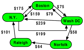
For example, suppose that we wanted to construct this graph denoting an airline’s pricing for flying from one city to another.

struct Flight {  // data for edges
    int price; // in dollars
};

struct Airport { // data for vertices
    string city;
};

typedef boost::adjacency_list<boost::listS, // store edges in lists
                             boost::vecS, // store vertices in a vector
                     boost::bidirectionalS, // a directed graph
                     Airport,  // vertex data
                     Flight    // edge data
                     >
                                AirlineGraph;
AirlineGraph ag(5);

cout << "We are in " << ag[v].city << endl;

and whenever we have an edge, e, we can access its data similarly:

ag[e].price = ag[e].price + 50; // price hike

enum Cities {Boston, NY, WashDC, Norfolk, Raleigh, endofCities};
std::array<string,5> cityNames {"Boston", "NY", "WashDC",
                                "Norfolk", "Raleigh"};
typedef pair<Cities, Cities> cpair;
pair<Cities, Cities> flights[]  {
       cpair(NY, Boston), cpair(NY, WashDC),
       cpair(Boston, NY), cpair(Boston, WashDC),
       cpair(WashDC, Boston), cpair(WashDC, NY), cpair(WashDC, Norfolk),
       cpair(Norfolk, Raleigh),
       cpair(Raleigh, NY)
};
int prices[] {
    175, 199,
    159, 75,
    79, 239, 58,
    64,
    101,
    -1 // stop value
};
AirlineGraph ag(5);
for (Cities i = Boston; i != endofCities; i = Cities(i+1))
{
    ag[(Vertex)i].city = cityNames[i];
}
for (int i = 0; prices[i] >= 0; ++i)
{
    auto e = add_edge ((Vertex)flights[i].first,
                    (Vertex)flights[i].second,
                 ag).first;
    ag[e].price = prices[i];
}

1.5.2 Temporary Data

If we want to associate data temporarily with either vertices or edges, we need to set up something like a map that would let us retrieve and store data values by vertex or edge.

The usual method for doing this would be to use an unordered_map. The Boost library provides hash functions for both vertices and edges, so we can define maps with those as keys, e.g.:

std::unordered_map<Vertex, bool, boost::hash<Vertex> > processed;
std::unordered_map<Edge, double, boost::hash<Edge> > distances;

For example, suppose that we wanted to temporarily label each vertex in a graph g with a boolean indicating whether it had been processed or not, initially set to false.

auto allVertices = vertices(g); // a pair of iterators
int nVertices = num_vertices(g);
vector<bool> processed (nVertices, false);
   ⋮
if (!processed[v])
{
    doSomethingToVertex(v);
    processed[v] = true;
}
   ⋮

2 Traversing a Graph

Many problems require us to visit all the vertices of a graph.

• For that we can use the vertices(g) iterators.

Very often, however, we want to visit all of the vertices that can be reached from some starting vertex.

• We can adapt some of the traversal techniques that we learned for trees.
• This will yield the “depth-first” and “breadth-first” traversals for graphs.

  • Both of these traversals will, in effect, discover a “tree” embedded in the graph.

2.1 Spanning Trees

A spanning tree for a connected graph $G=(V,E)$ is a graph $G’=(V,E’)$ such that $E’ \subseteq E$ and $G’$ is a tree. The spanning tree is a tree that is “embedded” in the graph.

• They are useful when we need to do something with each vertex, but using as few edges as possible.

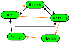
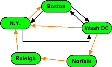
Question:
Is the set of vertices and orange edges shown here a spanning tree for the entire graph? If so, what is its root?

• No.

• Yes. The root is Boston

• Yes. The root is N.Y.

• Yes. The root is Norfolk

• Yes. The root is Raleigh

• Yes. The root is Wash DC

Question:
Is the set of vertices and orange edges shown here a spanning tree for the entire graph? If so, what is its root?

• No.

• Yes. The root is Boston

• Yes. The root is N.Y.

• Yes. The root is Norfolk

• Yes. The root is Raleigh

• Yes. The root is Wash DC

2.2 Depth-First Traversals - Trees

Consider the problem of searching a general tree for a given node.

• In a depth-first traversal, we investigate one child’s descendants before exploring its right siblings.

• In a breadth-first traversal, we explore all nodes at the same depth before moving on to any deeper nodes.

Most of the tree traversals that we looked at (prefix, postfix, and infix) were all variations of the depth-first idea.

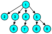
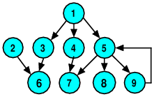
Question: In what order would a depth-first tree traversal, starting from node 1, visit these nodes? (Assume that children of the same node are processed in increasing numeric order.)

• 1 2 3 4 5 6 7 8 9

• 1 2 3 6 4 7 5 8 9

• 2 3 6 1 4 7 8 5 9

• None of the above.

void depthFirst (TreeNode* t)
{
  if (t != 0)
     for (int i = 0; i < t->numChildren; ++i)
        depthFirst (t->child[i]);
}

We convert this into a preorder or postorder process depending upon whether we process a node before or after visiting its children.

2.3 Depth-First Traversals of Graphs

Now, if we apply this same idea to a graph instead of a tree, starting with vertex 1:

void depthFirst (Graph& dg, Vertex v)
{
  auto edgeRange = out_edges(v, dg);
  for (auto e = edgeRange.first; 
       e != edgeRange.second; ++e)
     {
       Vertex w = target(*e, dg);
       depthFirst (dg, w);
     }
}

we can see some problems:

• Vertex 7 will be visited once as a “child” of 4, and visited again when we reach vertex 5.

• Worst of all, we will eventually go from 5 to 9, from 9 back to 5, then to 9 again, and so on, recursing forever (or until we run out of memory for the activation stack).

2.3.1 Using Sets to Cope with Cycles

We can adapt the tree algorithm for use in graphs by using some sort of data structure to keep track of which nodes have already been visited:

void depthFirst (Graph& dg, Vertex v, set<Vertex>& visited)
{
  visited.insert (v);
  auto edgeRange = out_edges(v, g);
  for (auto e = edgeRange.first; 
       e != edgeRange.second; ++e)
     {
       Vertex w = target(*e, dg);
       if (visited.count(w) == 0)
         depthFirst (dg, w, visited);
     }
}

The visited set records the vertices that we have already seen. When we are examining adjacent vertices to recursively visit, we simply pass over any that we have already visited.

2.4 Breadth-First Traversal of Trees

Breadth-first visits each node at the same depth (distance from the starting node) before moving on to more distant nodes.

In trees, this is also called “Level-Order” traversal.

Question: In what order would a breadth-first tree traversal, starting from node 1, visit these nodes?

• 1 2 3 4 5 6 7 8 9

• 1 2 3 6 4 7 5 8 9

• 2 3 6 1 4 7 8 5 9

• None of the above.

void breadthFirst (TreeNode* root)
{
   queue<TreeNode*, list<TreeNode*> > q;
   q.push (root);
   while (!q.empty())
     {
      v = q.front ();
      q.pop ();
      for (int i = 0; i < v->numChildren(); ++i)
        {
         TreeNode* w = v->child[i];
         if (w != 0)
           q.push (w);
        }
     }
}

We use a queue to receive the list of vertices to be visited, starting with the root, then the root’s children, then the root’s grandchildren, and so on.

2.5 Breadth-First Traversal of Graphs

Again, that tree code would have problems (including going into an infinite loop) if applied to more general graphs.

But we can use the same idea of a set of already-visited vertices to adapt this idea to traversing graphs.