  | 1 of 80


 |   |
| | 1 of 80
| |
Suppose you have to design a brand-new algorithm to do something never done before. You could start from scratch, given the problem statement and a programming language textbook, and you might come up with something useful.
A first question we might ask about any algorithm is how it manages to process multiple “pieces” of data:
Iterative: algorithms that work by looping
Recursive: algorithms that call themselves (directly or indirectly)
Among both iterative and recursive algorithms, we recognize some algorithms by an underlying “idea” of how they work:
Generic
Divide and conquer
Generate and test
Backtracking
Convergent
Dynamic programming
Now let’s look at some common forms of both iterative and recursive algorithms.
Perhaps the most widely recognized algorithmic style is “divide and conquer”. In this approach to design, a problem is broken into two or more smaller sub-problems, the sub-problems are solved, and the resulting sub-problem solutions are recombined into a whole solution.
Examples of divide and conquer that we have seen include the binary search, merge sort, and quick sort.
One of the most recent categories of algorithms to be recognized, generic algorithms are those that use a general-purpose “iterator” interface to process a range of data that could, in fact, be residing in almost any kind of container.
template <class InputIterator,
          class OutputIterator>
OutputIterator copy(InputIterator first,
                    InputIterator last,
                    OutputIterator result)
{
  while (first != last)
    {
      *result = *first;
      result++; first++;
    }
  return result;
}
In fact, the STL (standard template library), that eventually became part of the C++ standard library, was originally constructed as a showcase for the idea of generic programming.
A “generate and test” algorithm uses some relatively quick process to produce a series of “guesses” as to the appropriate solution, then tests each guess in turn to see if it is, in fact, a solution.
You can see generate and test in action in this code for producing random permutations.
//
//  Generate a random permutation of the integers from
//  0 .. n-1, storing the results in array a.
//
void permute1 (int a[], int n)
{
  for (int i = 0; i < n; i++)
    {
      a[i] = rnd(n);
      while (find(a,a+i,a[i]) != a+i)
         a[i] = rnd(n);
    }
}
The random numbers are used to generate a possible value for the $i^{\mbox{th}}$ number in the permutation.
Then a search is used to test and see if that number has already been used.
Generate-and-test is often used as a fall-back when we can’t come up with a better algorithm.
A variation of generate-and-test is backtracking. Backtracking is a technique that can be applied to problems where you have a large, but finite number of variables, each of which may take on a number of discrete values, and there is some overall test to decide if the entire set of assignments represents an acceptable solution.
An example of backtracking can be seen in the solution technique many people take to problems like this:
There are 3 adjacent houses, one red, one blue, and one green on Elm St. Each is occupied by a single person, and each has a garden with one kind of flower.
Bob does not live in the green house.
Pat lives between Bob and Sue.
Sue planted daisies.
Lilies are planted at the blue house.
The leftmost house has roses.
List the colors of the houses, the occupants, and their flowers, from left to right.
One way to approach this is to make a grid:
| left | middle | right | |
|---|---|---|---|
| House | |||
| Flowers | |||
| Person |
and list the possible values for each row:
| left | middle | right | |
|---|---|---|---|
| House (blue, green, red) | |||
| Flowers (daisies, lilies, roses) | |||
| Person (Bob, Pat, Sue) |
Now, try assigning values in each slot, until a contradiction is reached with one of the rules.
Let’s guess that the leftmost house is Blue:
| left | middle | right | |
|---|---|---|---|
| House (blue, green, red) | blue | ||
| Flowers (daisies, lilies, roses) | |||
| Person (Bob, Pat, Sue) |
and the middle one Green
| left | middle | right | |
|---|---|---|---|
| House (blue, green, red) | blue | green | |
| Flowers (daisies, lilies, roses) | |||
| Person (Bob, Pat, Sue) |
and the right one Red:
| left | middle | right | |
|---|---|---|---|
| House (blue, green, red) | blue | green | red |
| Flowers (daisies, lilies, roses) | |||
| Person (Bob, Pat, Sue) |
None of these lead to any contradictions with the rules. So let’s move on to the next row.
Let’s put daisies in the leftmost house.
| left | middle | right | |
|---|---|---|---|
| House (blue, green, red) | blue | green | red |
| Flowers (daisies, lilies, roses) | daisies | ||
| Person (Bob, Pat, Sue) |
Now we have our first contradiction. Rule 4 says that lilies are planted at the blue house and rule 5 says that the leftmost house has roses. So what do we do? We retract our most recent guess, and try a different value for that same slot.
Sticking with alphabetic order, we try lilies:
| left | middle | right | |
|---|---|---|---|
| House (blue, green, red) | blue | green | red |
| Flowers (daisies, lilies, roses) | lilies | ||
| Person (Bob, Pat, Sue) |
Again, a contradiction (rule 5). So we retract that guess and try roses.
| left | middle | right | |
|---|---|---|---|
| House (blue, green, red) | blue | green | red |
| Flowers (daisies, lilies, roses) | roses | ||
| Person (Bob, Pat, Sue) |
But that contradicts rule 4 (Lilies are planted at the blue house.). Now we have tried all possible kinds of flowers at this position. Since none of them work, we know that one of our earlier decisions has already precluded any possible solution. Which one? We’re probably not sure. So we retract our guess and backtrack to the slot before this one and try something else.
| left | middle | right | |
|---|---|---|---|
| House (blue, green, red) | blue | green | red |
| Flowers (daisies, lilies, roses) | |||
| Person (Bob, Pat, Sue) |
But we have no open alternatives for the color of the rightmost house, either. So we retract that guess and backtrack again:
| left | middle | right | |
|---|---|---|---|
| House (blue, green, red) | blue | green | |
| Flowers (daisies, lilies, roses) | |||
| Person (Bob, Pat, Sue) |
Here we can try a different possibility:
Maybe the middle house is red.
| left | middle | right | |
|---|---|---|---|
| House (blue, green, red) | blue | red | |
| Flowers (daisies, lilies, roses) | |||
| Person (Bob, Pat, Sue) |
and the rightmost house would have to be green.
| left | middle | right | |
|---|---|---|---|
| House (blue, green, red) | blue | red | green |
| Flowers (daisies, lilies, roses) | |||
| Person (Bob, Pat, Sue) |
You can probably see that this won’t work out either. Eventually we will have to back all the way up to our first decision, and try a different color for the leftmost house.
  | 1 of 12 |   |
Hopefully, you can see that, given enough time, this systematic approach would eventually arrive at a solution if one is possible, or would conclusively prove that no solution is possible.
We use backtracking largely in cases where we can’t find a more sophisticated way to arrive at a solution.
The essence of backtracking is:
Number the solution variables $[v_0, v_1, \ldots, v_{n-1}]$.
Number the possible values for each variable $[c_0, c_1, \ldots, c_{k-1}]$.
Start by assigning $c_0$ to each $v_i$.
If we have an acceptable solution, stop.
If the current solution is not acceptable, let i = n-1.
If i < 0, stop and signal that no solution is possible.
Let j be the index of the value assigned to variable $v_i$ (i.e., $v_i = c_j$). If $j < k-1$, assign $c_{j+1}$ to $v_i$ and go back to step 4.
But if $j \geq k-1$, assign $c_0$ to $v_i$, decrement i, and go back to step 6.
There are lots of variations possible. It’s fairly easy to modify this scheme to deal with situations where different variables have different sets of possible values.
Many game-playing programs use a form of this kind of backtracking to select the computer’s move.
There are 9 variables in this problem: colorL, colorM, colorR, flowersL, flowersM, flowersR, personL, personM, and personR, where the “L”, “M”, and “R” subscripts denote “left”, “Middle”, and “Right”, respectively.
Each can take on 3 possible values. Letting blue=daisies=Bob=0, green=lilies=Pat=1, and red=roses=Sue=2, we can represent our progress through the problem like this:
Start with none of the variables assigned.
| colorL | colorM | colorR | flowersL | flowersM | flowersR | personL | personM | personR |
|---|---|---|---|---|---|---|---|---|
Then assign red to the left house:
| colorL | colorM | colorR | flowersL | flowersM | flowersR | personL | personM | personR |
|---|---|---|---|---|---|---|---|---|
| 0 |
and green to the middle house:
| colorL | colorM | colorR | flowersL | flowersM | flowersR | personL | personM | personR |
|---|---|---|---|---|---|---|---|---|
| 0 | 1 |
Continuing on, we can show the whole progress (up to the point where we stopped earlier), showing each step as a separate line:
| colorL | colorM | colorR | flowersL | flowersM | flowersR | personL | personM | personR |
|---|---|---|---|---|---|---|---|---|
| 0 | ||||||||
| 0 | 1 | |||||||
| 0 | 1 | 2 | ||||||
| 0 | 1 | 2 | 0 | |||||
| 0 | 1 | 2 | 1 | |||||
| 0 | 1 | 2 | 2 | |||||
| 0 | 2 | |||||||
| 0 | 2 | 1 |
and so on.
Actually, even here we may have played fast and loose a little with the rules. How did we know that the middle house should start with color 1 instead of 0? Only because there is an implicit rule saying that there can only be a single house of each color. A violation of that rule is just another contradiction, so we could actually argue that the steps we went through were:
| colorL | colorM | colorR | flowersL | flowersM | flowersR | personL | personM | personR |
|---|---|---|---|---|---|---|---|---|
| 0 | ||||||||
| 0 | 0 | |||||||
| 0 | 1 | |||||||
| 0 | 1 | 0 | ||||||
| 0 | 1 | 1 | ||||||
| 0 | 1 | 2 | ||||||
| 0 | 1 | 2 | 0 | |||||
| 0 | 1 | 2 | 1 | |||||
| 0 | 1 | 2 | 2 | |||||
| 0 | 2 | |||||||
| 0 | 2 | 0 | ||||||
| 0 | 2 | 1 |
and so on. This is more typical of how we would be likely to program a solution.
| | 1 of 6 | |
Here’s another way to think about this process.
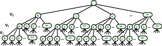
This tree shows the “solution space” for a backtracking problem. At one level is the first problem variable with all of its possible solution values. Each node at the first level represents a possible value for the variable $v_0$.
The traditional way to program backtracking has been to write a recursive function to search this solution space. The first call deals with possible values for $v_0$, and loops through each one in turn. For each possible value of $v_0$, we recursively call the same routine, but instruct it to work with $v_1$ instead of $v_0$. That recursive call will loop through all possible values of $v_1$, trying each one and then recursively calling itself with instructions to work on $v_2$, and so on.
The CS Dept. has a list of courses to offer next semester, and a list of available time slots in which to place them.
Some courses “conflict” – they cannot be scheduled at the same time because
students may want to take both courses in the same semester
the same faculty member is teaching both.
Suppose that the classes are numbered 0 ... NumClasses-1, and that the time slots are numbered 0 ... NumTimes-1.
We will assume that someone has already written a function
bool conflicts(int class1, int class2);
to determine if two classes conflict.
Our job is to write the function that actually does the scheduling. We will store the schedule in
vector<int> timeOfClass (numClasses, -1);
so that timeOfClass[c] is the time slot in which class c has been scheduled (-1 indicates that we have not yet assigned a time to c).
We start by defining a utility function, noConflicts, to determine if it’s OK to assign a given class to a given time slot.
bool noConflicts (int class, int time)
// Would assigning the given class to the given time
// cause a conflict with any already scheduled classes?
// Return true if no conflicts would be caused.
{
  for (int c = 0; c < class; ++c)
    {
     if (timeOfClass[c] = time   // if c is already schedule at this time
         && conflicts(c, class)) // and c conflicts with class
       return false;             // then we can't schedule class at this time
    }
  return true;
}
noConflicts simply examines every other class already in this time slot to see if it conflicts with this one.
Here, then, is the main scheduling algorithm. schedule(i) returns true if it is able to schedule all the classes from i ... numClasses-1.
bool schedule(int class)
{
  if (class == NumClasses)
    return true;
  else
    for (int t = 1; t <= NumTimes; ++t)
      {
       if (noConflicts(class, t))
         {
          timeOfClass[class] = t;
          if (schedule(i+1)) return true;
         }
      }
  timeOfClass[class] = -1;
  return false;    // all choices failed
}
It does this by trying every plausible time slot for class i until it finds one that allows all the remaining classes to be (recursively) scheduled.
If it can’t find a slot in which to place class i, it returns false.
Whenever a recursive call from schedule returns false back to an earlier call of itself, the earlier call is forced to try a different time slot for a previously scheduled class.
Analysis:
noConflicts() is $O(\mbox{class})$.
bool noConflicts (int class, int time)
// Would assigning the given class to the given time
// cause a conflict with any already scheduled classes?
// Return true if no conflicts would be caused.
{
  for (int c = 0; c < class; ++c)
    {
     if (timeOfClass[c] = time
         && conflicts(c, class))
       return false;
    }
  return true;
}
bool schedule(int class)
{
  if (class == NumClasses)
    return true;
  else
    for (int t = 1; t <= NumTimes; ++t)
      {
       if (noConflicts(class, t))
         {
          timeOfClass[class] = t;
          if (schedule(i+1)) return true;
         }
      }
  timeOfClass[class] = -1;
  return false;    // all choices failed
}
The worst case of schedule() occurs when no schedule is possible.
NumTimes possibilities.NumTimes possibilities of its own, for a total of $\mbox{NumTimes}^2$ possibilities for the two classes.Each try involves a call to noConflicts, so the overall algorithm is $O\left(\mbox{NumClasses}*\mbox{NumTimes}^{\mbox{NumClasses}}\right)$.
We say that this routine is exponential in
NumClasses. Such exponential growth is worse, for sufficiently large inputs, than any polynomial big-O().
Can we do this without the recursion?
Yes.
Let’s return again to the tree view of the possible solutions to a backtracking problem.
Let’s assume our tree has 5 levels, corresponding to $v_0$ through $v_4$, and that each variable can take on any of 3 values.
Now, suppose we list the possible solutions from left to right in this tree, listing each one from $v_{n-1}$ down to $v_0$.
So, if we had an ADT for counting N digit numbers in an arbitrary base, we could use that as a kind of generator for backtracking solutions.
The code shown here represents a backtracking state generator.
class BackTrack {
public:
  BackTrack (unsigned nVariables, unsigned arity=2);
  // Create a backtracking state for a problem with
  // nVariables variables, each of which has the same
  // number of possible values (arity).

  template <class Iterator>
  BackTrack (Iterator arityBegin,
             Iterator arityEnd);
  // Create a backtracking state in which each variable may have
  // a different number of possible values. The values are obtained
  // as integers stored in positions arityBegin .. arityEnd as per
  // the usual conventions for C++ iterators. The number of
  // variables in the system are inferred from the number of
  // positions in the given range.

  unsigned operator[] (unsigned variableNumber) const;
  // Returns the current value associated with the indicated
  // variable.

  unsigned numberOfVariables() const;
  // Returns the number of variables in the backtracking system.

  unsigned arity (unsigned variableNumber) const;
  // Returns the number of potential values that can be assigned
  // to the indicated variable.

  bool more() const;
  // Indicates whether additional candidate solutions exist that
  // can be reached by subsequent ++ or prune operations.

  void prune (unsigned level);
  // Indicates that the combination of values associated with
  // variables 0 .. level-1 (inclusive) has been judged unacceptable
  // (regardless of the values that could be given to variables
  // level..numberOfVariables()-1.  The backtracking state will advance
  // to the next solution in which at least one of the values in the
  // variables 0..level-1 will have changed.

  BackTrack& operator++();
  // Indicates that the combination of values associated with
  // variables 0 .. nVariables-1 (inclusive) has been judged unacceptable.
  // The backtracking state will advance
  // to the next solution in which at least one of the values in the
  // variables 0..level-1 will have changed.

  BackTrack operator++(int);
  // Same as other operator++, but returns a copy of the old backtrack state

private:
  bool done;
  vector<unsigned> arities;
  vector<unsigned> values;

};
The constructors allow us to indicate how many variables we need and what the “arity” (number of possible values) for them are. For example
BackTrack problem(9, 3);
would create backtracking state problem with 9 variables, each of which can take on the values 0, 1, or 2.
The current value of any variable can be read using the square brackets operator:
cout << "Variable " << i
     << " has value " << problem[i]
     << endl;
We can advance to the next possible state using the ++ operator, and the more() function tells us if we have tried every possible combination. For example, if we were to simply loop through all possible states:
BackTrack problem(4, 3);
// 4 questions, each with 3 possible answers
while (problem.more())
 {
   for (int i = 0; i < 4; ++i)
     cout << problem[i] << ' ';
   cout << endl;
   ++problem;
 }
the output would be: 0000, 0001, 0002, 0010, 0011, 0012, 0020, 0021, 0022, 0100, … , 2222.
A typical backtracking problem can then be solved this way:
BackTrack problem(nVariables, nValues);
bool solved = false;
while ((!solved) && problem.more())
 {
   solved = checkSolution(problem);

   if (!solved)
     ++problem;
 }
where checkSolution is a function that returns true if the current problem state is an acceptable solution.
Let’s look at how to use this class to solve the 3-houses puzzle. In this puzzle, we have a total of 9 variables. We give them names here, assigning those names to the integers from 0 to 8.
enum Questions {colorOfHouse1=0,
                colorOfHouse2=1,
                colorOfHouse3=2,
                flowersAtHouse1=3,
                flowersAtHouse2=4,
                flowersAtHouse3=5,
                occupantOfHouse1=6,
                occupantOfHouse2=7,
                occupantOfHouse3=8};
Although each group of three variables represents something different, it so happens that all the variables can take on three possible values.
enum Colors {red=0, blue=1, green=2};
const char* colorNames[] = {"red", "blue", "green"};

enum Occupants {bob=0, pat=1, sue=2};
const char* occupantNames[] = {"Bob", "Pat", "Sue"};

enum Flowers {daisies=0, lilies=1, roses=2};
const char* flowerNames[] = {"daisies", "lilies", "roses"};
Again, we’ll give these descriptive names, but bind them to the integers 0, 1, and 2.
The related arrays of character strings are useful for output purposes:
void describeHouse(int houseNumber,
                   Occupants occupant,
                   Colors c, Flowers f)
{
  cout << occupantNames[occupant]
       << " lives in house " << houseNumber
       << ", which is painted " << colorNames[c]
       << " and has "
       << flowerNames[f] << endl;
}
Now we’re ready to set up the main routine for the solution. This just adds a bit of output to the basic solution loop.
int main()
{
  BackTrack problem(9, 3);
    // 9 questions, each with 3 possible answers
  bool solved = false;
  while ((!solved) && problem.more())
    {
      for (int i = 0; i < 9; ++i)
        cout << problem[i] << ' ';
      cout << endl;

      solved = checkSolution(problem);

      if (!solved)
        ++problem;
    }

  if (solved)
    {
      describeHouse(1,
                    (Occupants)problem[occupantOfHouse1],
                    (Colors)problem[colorOfHouse1],
                    (Flowers)problem[flowersAtHouse1]);
      describeHouse(2,
                    (Occupants)problem[occupantOfHouse2],
                    (Colors)problem[colorOfHouse2],
                    (Flowers)problem[flowersAtHouse2]);
      describeHouse(3,
                    (Occupants)problem[occupantOfHouse3],
                    (Colors)problem[colorOfHouse3],
                    (Flowers)problem[flowersAtHouse3]);
    }
  else
    cout << "Problem has no solution" << endl;
}
Of course, all the “good stuff” is in the checkSolution function - that’s where we have to determine whether the current set of numbers represent a possible solution to the puzzle or not.
We’ll take this in stages.
bool checkSolution(const BackTrack& bt)
  // Check the state of bt to see if it
  //   represents a valid solution.
{
  bool OK = true;

  // Implicit rule: each house is different
  if (bt[occupantOfHouse1] == bt[occupantOfHouse2])
    OK = false;
  if (bt[occupantOfHouse1] == bt[occupantOfHouse3])
    OK = false;
  if (bt[occupantOfHouse2] == bt[occupantOfHouse3])
    OK = false;
     ⋮
OK will represent the result of our tests overall. It starts out true but will be set to false the moment we find a contradiction between the current problem state and the rules of the puzzle.
The first rules to be checked are implicit ones. Bob can’t live in more than one house in this problem, and neither can Sue or Pat. So if any two houses have the same occupant, set OK to false. Note that bt[occupantOfHouse1] denotes the current assignment, in bt, to the occupantOfHouse1 variable. It will either be bob (0), pat (1), or sue (2).
We have similar rules for the house colors and the flowers.
⋮
  if (bt[colorOfHouse1] == bt[colorOfHouse2])
    OK = false;
  if (bt[colorOfHouse1] == bt[colorOfHouse3])
    OK = false;
  if (bt[colorOfHouse2] == bt[colorOfHouse3])
    OK = false;

  if (bt[flowersAtHouse1] == bt[flowersAtHouse2])
    OK = false;
  if (bt[flowersAtHouse1] == bt[flowersAtHouse3])
    OK = false;
  if (bt[flowersAtHouse2] == bt[flowersAtHouse3])
    OK = false;
    ⋮
⋮
  // 1. Bob does not live in the green house.
  int bobsHouse = indexOf(bt, bob,
                          occupantOfHouse1,
                          occupantOfHouse2,
                          occupantOfHouse3);
  int greenHouse = indexOf(bt, green,
                          colorOfHouse1,
                          colorOfHouse2,
                           colorOfHouse3);

  if (bobsHouse - occupantOfHouse1
      == greenHouse - colorOfHouse1)
    OK = false;
    ⋮
Now we’re ready to consider the explicit rules of the puzzle. For rule 1, we need to know which house bob lives in and which house is green.
We’ll need to do a lot of this kind of lookup in this function, so we’ll introduce a utility function, indexOf, that tells us which of three variable numbers contains a desired value.
int indexOf (const BackTrack& bt, int value,
             int candidate1, int candidate2,
             int candidate3)
{
  if (bt[candidate1] == value)
    return candidate1;
  else if (bt[candidate2] == value)
    return candidate2;
  else
    return candidate3;
}
⋮
  // 2. Pat lives between Bob and Sue.
  if (bt[occupantOfHouse2] != pat)
    OK = false;
    ⋮
The next rule is easy. If Pat lives between them, Pat must be in the second house.
The code for the third rule looks much like the code for the first rule.
⋮
  // 3. Sue planted daisies.
  int suesHouse = indexOf(bt, sue,
                          occupantOfHouse1,
                          occupantOfHouse2,
                          occupantOfHouse3);
  int daisiesHouse = indexOf(bt, daisies,
                             flowersAtHouse1,
                             flowersAtHouse2,
                             flowersAtHouse3);

  if (suesHouse - occupantOfHouse1 != daisiesHouse - flowersAtHouse1)
    OK = false;
    ⋮
⋮
  // 4. Lilies are planted at the blue house.
  int liliesHouse = indexOf(bt, lilies,
                            flowersAtHouse1,
                            flowersAtHouse2,
                            flowersAtHouse3);
  int blueHouse = indexOf(bt, blue,
                          colorOfHouse1,
                          colorOfHouse2,
                          colorOfHouse3);

  if (liliesHouse - flowersAtHouse1
      != blueHouse - colorOfHouse1)
    OK = false;
    ⋮
And so does the 4th rule.
⋮
  // 5. The leftmost house has roses.
  if (bt[flowersAtHouse1] != roses)
    OK = false;

  return OK;
}
And the fifth and final rule is easy.
If we throw all this together and run it we would see the following output:
0 0 0 0 0 0 0 0 0
0 0 0 0 0 0 0 0 1
0 0 0 0 0 0 0 0 2
0 0 0 0 0 0 0 1 0
0 0 0 0 0 0 0 1 1
0 0 0 0 0 0 0 1 2
0 0 0 0 0 0 0 2 0
0 0 0 0 0 0 0 2 1
0 0 0 0 0 0 0 2 2
0 0 0 0 0 0 1 0 0
    ⋮
… and, about 4000 lines later …
    ⋮
0 1 2 2 1 0 0 0 2
0 1 2 2 1 0 0 1 0
0 1 2 2 1 0 0 1 1
0 1 2 2 1 0 0 1 2
Bob lives in house 1, which is painted red and has roses
Pat lives in house 2, which is painted blue and has lilies
Sue lives in house 3, which is painted green and has daisies
Backtracking, despite its exponential-time behavior, continues to arise in problems for which no better solution method is known. A lot of effort goes into finding ways to speed up its average performance.
One of the most common improvements is to use an some kind of “early” test to determine if a particular assignment to a particular variable is plausible rather than always waiting until all variables have been assigned to do any checking.
Again, if we think of the set of possible solutions in terms of a tree, as shown here, then the use of these early “plausibility” tests may have the effect of pruning entire branches of the tree, meaning that we don’t actually need to explore all those alternatives.
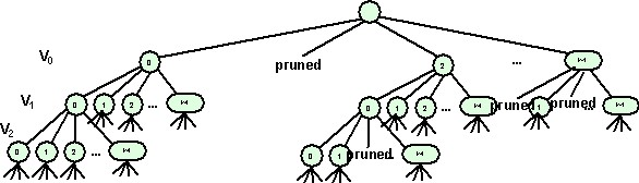
Note that the effect of “pruning” is most significant when it can occur early in the tree. A lot of research and design effort has gone into ideas like trying to reorder the variables and/or values so that pruning will occur as early as possible.
Our backtracking state generator can easily accommodate pruning.
class BackTrack {
public:
  ⋮
  void prune (unsigned level);
  // Indicates that the combination of values associated with
  // variables 0 .. level-1 (inclusive) has been judged unacceptable
  // (regardless of the values that could be given to variables
  // level..numberOfVariables()-1.  The backtracking state will
  // advance to the next solution in which at least one of the
  // values in the variables 0..level-1 will have changed.
  ⋮
In fact, the “normal” ++ operator is actually implemented as prune(numberOfVariables()) (which is no pruning at all.)
Let’s look, briefly, at just how the backtracking generator works.
class BackTrack {
public:
  ⋮
private:
  bool done;
  vector<unsigned> arities;
  vector<unsigned> values;
};
We use a vector to hold the current values for all of our variables. We also have a vector, arities, that indicates the number of different values each variable can take on.
In the problems we have been looking at, all the variables have the same arity, but this isn’t true for all backtracking problems.
When we create a new backtracking state, we start with all the variable values set to zero.
BackTrack::BackTrack (unsigned nVariables, unsigned arity=2)
  // Create a backtracking state for a problem with
  // nVariables variables, each of which has the same
  // number of possible values (arity).
  : arities(nVariables, arity),  values(nVariables, 0), done(false)
{
}
Pruning is accomplished by treating variables 0 … level-1 as a level-digit number, adding 1 to it using the same “add and carry to the left” procedure you learned in grade-school arithmetic.
void BackTrack::prune (unsigned level)
  // Indicates that the combination of values associated with
  // variables 0 .. level-1 (inclusive) has been judged unacceptable
  // (regardless of the values that could be given to variables
  // level..numberOfVariables()-1.  The backtracking state will advance
  // to the next solution in which at least one of the values in the
  // variables 0..level-1 will have changed.
{
  level = (level > numberOfVariables()) ? numberOfVariables() : level;
  fill (values.begin()+level, values.end(), 0);


  // Treat the top level-1 values as a level-1 digit number. Add one
  // to the rightmost "digit". If this digit goes too high, reset it to
  // zero and "carry one to the left".
  int k = level-1;
  bool carry = true;
  while (k >= 0 && carry)
    {
      values[k] += 1;
      if (values[k] >= arities[k])
        values[k] = 0;
      else
        carry = false;
      --k;
    }
  done = carry;
}
The variables being “pruned”, the ones in positions level … numberOfVariables(), are simply set to zero.
The normal ++ is simply a special case in which no variables are actually pruned, but the state is advanced to the next “number”.
BackTrack& BackTrack::operator++()
  // Indicates that the combination of values associated with
  // variables 0 .. nVariables-1 (inclusive) has been judged unacceptable.
  // The backtracking state will advance
  // to the next solution in which at least one of the values in the
  // variables 0..level-1 will have changed.
{
  prune(numberOfVariables());
  return *this;
}
Applying Pruning
Now, to actually use pruning in a problem requires a bit more effort when we check the solution state. Instead of simply indicating whether the state is acceptable, we now want to indicate the smallest variable number that we want to change. Basically, for any rule that involves variables $v_j$ and $v_k$, if we find that the rule is violated, then the larger of j or k will need to be changed next.
Instead of a simple boolean OK variable, we now use an integer to track the variable that we want changed on the next step.
int checkSolution(const BackTrack& bt)
  // Check the state of bt to see if it represents a valid solution.
  // Return -1 if a solution. If not a solution, return the smallest
  // number of any problem variable known to be incorrect.
{
  int knownIncorrect = bt.numberOfVariables();

  // Implicit rule: each house is different
  if (bt[occupantOfHouse1] == bt[occupantOfHouse2])
    knownIncorrect = min(knownIncorrect,
                       max(occupantOfHouse1, occupantOfHouse2));
    ⋮
If we fail the test, we replace that integer with the larger of the variable numbers involved in the test, provided that we haven’t already found a lower-numbered variable for pruning.
The same pattern gets repeated many times for the implicit rules.
⋮
  if (bt[occupantOfHouse1] == bt[occupantOfHouse3])
    knownIncorrect = min(knownIncorrect,
                         max(occupantOfHouse1,
                             occupantOfHouse3));
  if (bt[occupantOfHouse2] == bt[occupantOfHouse3])
    knownIncorrect = min(knownIncorrect,
                         max(occupantOfHouse2,
                             occupantOfHouse3));
    ⋮
and for the explicit rules as well.
⋮
  // 1. Bob does not live in the green house.
  int bobsHouse = indexOf(bt, bob,
                          occupantOfHouse1,
                          occupantOfHouse2,
                          occupantOfHouse3);
  int greenHouse = indexOf(bt, green,
                          colorOfHouse1,
                          colorOfHouse2,
                           colorOfHouse3);

  if (bobsHouse - occupantOfHouse1 == greenHouse - colorOfHouse1)
    knownIncorrect = min(knownIncorrect,
                         max(bobsHouse, greenHouse));


  // 2. Pat lives between Bob and Sue.
  if (bt[occupantOfHouse2] != pat)
    knownIncorrect = min(knownIncorrect, occupantOfHouse2);
    ⋮
until we have checked all the rules and are ready to return.
⋮
  if (knownIncorrect >= bt.numberOfVariables())
    return -1;
  else
    return knownIncorrect;
}
BackTrack problem(9, 3);
    // 9 questions, each with 3 possible answers
  bool solved = false;
  while ((!solved) && problem.more())
    {
      for (int i = 0; i < 9; ++i)
        cout << problem[i] << ' ';
      cout << endl;

      int pruneAt = checkSolution(problem);
      if (pruneAt < 0)
        solved = true;
      else
        problem.prune(pruneAt+1);
    }
The main program loop now is altered to use prune instead of ++.
If we run this version, the output is
0 0 0 0 0 0 0 0 0
0 1 0 0 0 0 0 0 0
0 1 1 0 0 0 0 0 0
0 1 2 0 0 0 0 0 0
0 1 2 1 0 0 0 0 0
0 1 2 2 0 0 0 0 0
0 1 2 2 0 1 0 0 0
0 1 2 2 0 2 0 0 0
0 1 2 2 1 0 0 0 0
0 1 2 2 1 0 0 1 0
0 1 2 2 1 0 0 1 1
0 1 2 2 1 0 0 1 2
Bob lives in house 1, which is painted red and has roses
Pat lives in house 2, which is painted blue and has lilies
Sue lives in house 3, which is painted green and has daisies
That’s the whole thing! Only 12 potential solutions were examined, instead of more than 4000.
This shows that pruning can be critical to making backtracking work efficiently. But don’t get carried away. The amount of reduction you get from pruning varies considerably (we were probably a bit lucky here) and, even with pruning, the worst case is still exponential time.
In contrast to “generate-and-test”, some algorithms work by “generate-and-improve”. An initial guess is made at a solution, which is successively improved by some process that, it is hoped, eventually “converges” to the correct solution.
Convergent algorithms are most common in numerical processing. For example, the code shown here is a convergent algorithm for computing square roots, given an initial guess. [^ Calculus die-hards may recognize this as Newton’s Method.]
double sqrt (double x, double initialGuess)
{
  double root = initialGuess;
  do {
      double last = root;
      root = 0.5 * (root + x / root);
  } while (abs(root - last) > 0.0001);
  return root;
}
If we were to call, for example, sqrt(2.0,1.0) (find the square root of 2 using an initial guess of 1), the successive values of root would be: 1, 1.5, 1.416667, 1.414216, 1.414214, at which point the algorithm would return.
Many scientific and engineering programs depend upon convergent algorithms.
Dynamic programming is a replacement for recursion that is useful when a recursive solution would repeatedly solve the same small subproblems.
The basic idea is to go ahead and solve the smaller problems, but to save the results in a data structure so that, if you need the same subproblem solved again, you can just fetch the prior answer from the data structure.
Suppose we have a set of $n$ distinct items, and need to select $k$ of them at random (e.g., dealing 5 cards from a deck of 52). Assume that we aren’t concerned about the order in which we obtained the selected items, but we want to know how many different possible sets of items we could possible obtain.
The number of different combinations we can obtain by selecting k items from a set of n, without replacement, is written as $\left(\begin{array}{c} n \\ k \end{array} \right)$ or sometimes as $C(n,k)$.
It can be evaluated as
\[ C(n,n) = C(n,0) = 1 \]
\[ C(n,k) = C(n - 1, k - 1) + C(n - 1, k), \; 0 < k < n \]
A straightforward recursive solution would be the code shown here.
long C(int n, int k)
{
  if (k==0 || k==n)
    return 1;
  else
    return C(n-1,k-1) + C(n-1,k);
}
But this wastes effort re-evaluating smaller problem over and over again. For example,
\[ C(5,2) = C(4,1) + C(4,2) \]
No problem so far, but let’s expand each of the items on the right
\[ \begin{eqnarray*} C(4,1) & = & C(3,0) + C(3,1) \\ C(4,2) & = & C(3,1) + C(3,2) \end{eqnarray*} \]
and you can start to see that one subproblem $C(3,1)$ has already arisen in two different places.
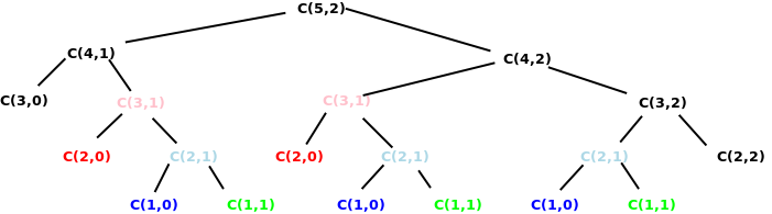
Furthermore, if we were to expand these again, we would find that both occurrences of $C(3,1)$ and $C(3,2)$ will need the value of $C(2,1)$. In fact, most of the run time of this algorithm will be devoted to solving and re-solving the same smaller problems, over and over.
Here is the full call tree for computing C(5,2). Note what a large fraction of the total number of calls are to repeated/dupicated parameters.
Reversing the Calculation
But wait — there’s more!
Those recursive calls, when they take place, always ask for the solution to a “smaller” problem (either n, or k, or both are smaller).
But in this problem, there are only so many possible smaller problems.
Because we never need the answer to a larger problem before we can answer a smaller one, we can turn the whole evaluation inside-out and simply start by evaluating the simple problems, then the larger problems that can be solved from those, and so on, until we reach the original problem that we were really interested in.
long C(int n, int k)
{
  Matrix<long> savedResults(n+1, k+1)
  for (int i = 0; i <= n; ++i)
     for (int j = 0; j <= k; ++j)
       savedResults(i,j) = -1;

  // Solve the easy problems first, working up towards
  //   the harder ones
  for (n1 = 1; n1 <= n; ++n1)
    {
      savedResults[n1][0] = 1;
      savedResults[n1][n1] = 1;
      for (int k1 = 1; k1 < n1; ++k1)
        savedResults(n1,k1) = savedResults(n1-1, k1-1) +
                               savedResults(n1-1, k1);
    }

  return savedResults(n, k);
}
And suddenly, there’s no recursion left at all!
This idea of computing and storing the results of all subproblems of the problem we really want to solve, in order from simplest/smallest up to the one we really want, is called dynamic programming.
Dynamic programming frequently not only prevents repeated recursion over common sub-problems, but often introduces a structure over which a purely iterative solution is possible.
One of the classic problems solvable by dynamic programming is computing the “edit distance” between two strings: the minimum number of single-character insertions, deletions, or replacements required to convert one string into another.
The edit distance can be used for such purposes as suggesting, in a spell checker, a list of plausible replacements for a misspelled word. For each word not found in the dictionary (and therefore presumably misspelled), list all words in the dictionary that are a small edit distance way from the misspelling.
We can compute the edit distance between two strings by working from the ends. The three operations available to us are
Add one character to the end of a string
Remove one character from the end of a string
Change the character at the end of a string.
Suppose, for example, that we wanted to compute the edit distance between “Zeil” and “trials” (make up your own joke here). Starting with “Zeil”, we consider what would have to be done to get “trials” if the last step taken were “add”, “remove”, or “change”, respectively:
If we knew how to convert “Zeil” to “trial”, we could add “s” to get the desired word.
If we knew how to convert “Zei” to “trials”, then we would actually have “trialsl” and we could remove that last character to get the desired word.
If we knew how to convert “Zei” to “trial”, then we would actually have “triall” and we could change the final “l” to “s” to get the desired word.
Notice that what we have done is to reduce the original problem to 3 “smaller” problems: convert “Zeil” to “trial”, or “Zei” to “trials”, or “Zei” to “trial”.
We continue, recursively, to break down these problems:
Convert “Zeil” to “trial”, then add “s” to get the desired word.
To convert “Zeil” to “trial”,
Convert “Zei” to “trials”, giving “trialsl”, then remove the last character.
To convert “Zei” to “trials”,
Convert “Zei” to “trial”, giving “triall”, then change the final “l” to “s”.
To convert “Zei” to “trial”,
Now we have nine subproblems to solve, but note that the strings involved are getting shorter. Eventually we will get down to subproblems involving an empty string, such as
Convert "" to "xyz",'
which can be trivially solved by a series of “Adds”.
Here you see the recursive implementation of the edit distance calculation.
int editDistance (string x, string y)
{
  if (x == "")
     return y.length(); // base case
  else if (y == "")
     return x.length(); // base case
  else
    {
      int addDistance = editDistance(x, y.substr(0,y.length()-1)) + 1;
      int removeDistance = editDistance(x.substr(0,x.length()-1), y) + 1;
      int changeDistance = editDistance(x.substr(0,x.length()-1),
                                        y.substr(0,y.length()-1))
        + (x[x.length()-1] == y[y.length()-1]) ? 0 : 1;
      return min(min(addDistance, removeDistance), changeDistance);
    }
}
In the main portion, we don’t know, off hand, whether the cheapest way to convert one string into another involves a final add, remove, or change, so we evaluate all three possibilities and return the minimum distance from among the three.
In each case, we recursively compute the distance (number of adds, removes, and changes) required to “set up” a final add, a final remove, or a final change. We add one to the add distance and the remove distance to account for the final add or remove. For the change distance, we add one only if the final characters in the strings are different (if not, no final change is required).
We can solve the same problem via dynamic programming by, again, reversing the direction so that we work the smaller subproblems first, keeping the answers in a table.
For example, in converting “Zeil” to “trials”, we start by forming a table of the cost (edit distance) to convert "“ to ”“, ”t“, ”tr“, ”tri", etc.:
| λ | t | r | i | a | l | s | |
|---|---|---|---|---|---|---|---|
| λ | 0 | 1 | 2 | 3 | 4 | 5 | 6 |
(The symbol λ denotes the empty string.)
In other words, we need 0 steps to convert "“ to ”“, 1 to convert ”“ to ”t“, 2 to convert ”“ to ”tr", and so on.
Next, we add a row to describe the cost of converting “Z” to "“, ”t“, ”tr“, … , ”trials":
| λ | t | r | i | a | l | s | |
|---|---|---|---|---|---|---|---|
| λ | 0 | 1 | 2 | 3 | 4 | 5 | 6 |
| Z | 1 | 1 | 2 | 3 | 4 | 5 | 6 |
OK, clearly we need 1 step to convert “Z” to "". How are the other entries in this row computed?
Looking Closer
Let’s back up just a bit:
| λ | t | r | i | a | l | s | |
|---|---|---|---|---|---|---|---|
| λ | 0 | 1 | 2 | 3 | 4 | 5 | 6 |
| Z | 1 | ? |
What’s the minimum cost to convert “Z” to “t”? It’s the smallest of the three values computed as
The last of these yields the minimal distance: 1.
Applying the General Rule
| λ | t | r | i | a | l | s | |
|---|---|---|---|---|---|---|---|
| λ | 0 | 1 | 2 | 3 | 4 | 5 | 6 |
| Z | 1 | 1 | ? |
What’s the minimum cost to convert “Z” to “tr”? It’s the smallest of the three values computed as
The last of these yields the minimal distance: 2.
Filling in the rest of the row:
| λ | t | r | i | a | l | s | |
|---|---|---|---|---|---|---|---|
| λ | 0 | 1 | 2 | 3 | 4 | 5 | 6 |
| Z | 1 | 1 | 2 | 3 | 4 | 5 | 6 |
Filling In The Table
And we add the next row, using the same technique:
| λ | t | r | i | a | l | s | |
|---|---|---|---|---|---|---|---|
| λ | 0 | 1 | 2 | 3 | 4 | 5 | 6 |
| Z | 1 | 1 | 2 | 3 | 4 | 5 | 6 |
| e | 2 | 2 | 2 | 3 | 4 | 5 | 6 |
The row after that becomes a bit more interesting. When we get this far …
| λ | t | r | i | a | l | s | |
|---|---|---|---|---|---|---|---|
| λ | 0 | 1 | 2 | 3 | 4 | 5 | 6 |
| Z | 1 | 1 | 2 | 3 | 4 | 5 | 6 |
| e | 2 | 2 | 2 | 3 | 4 | 5 | 6 |
| i | 3 | 3 | 3 | ? |
… we are looking at the cost of converting “Zei” to “tri”. It’s the smallest of the three values computed as
The last of these yields the minimal cost of 2.
| λ | t | r | i | a | l | s | |
|---|---|---|---|---|---|---|---|
| λ | 0 | 1 | 2 | 3 | 4 | 5 | 6 |
| Z | 1 | 1 | 2 | 3 | 4 | 5 | 6 |
| e | 2 | 2 | 2 | 3 | 4 | 5 | 6 |
| i | 3 | 3 | 3 | 2 | ? |
and then we can fill out the rest of the row:
| λ | t | r | i | a | l | s | |
|---|---|---|---|---|---|---|---|
| λ | 0 | 1 | 2 | 3 | 4 | 5 | 6 |
| Z | 1 | 1 | 2 | 3 | 4 | 5 | 6 |
| e | 2 | 2 | 2 | 3 | 4 | 5 | 6 |
| i | 3 | 3 | 3 | 2 | 3 | 4 | 5 |
and finally, the last row of the table:
| λ | t | r | i | a | l | s | |
|---|---|---|---|---|---|---|---|
| λ | 0 | 1 | 2 | 3 | 4 | 5 | 6 |
| Z | 1 | 1 | 2 | 3 | 4 | 5 | 6 |
| e | 2 | 2 | 2 | 3 | 4 | 5 | 6 |
| i | 3 | 3 | 3 | 2 | 3 | 4 | 5 |
| l | 4 | 4 | 4 | 3 | 3 | 3 | 4 |
Note that this last row, again, has a situation where the cost of a change is zero plus the subproblem cost, because the two characters involved are the same (“l”).
From the lower right hand corner, then, we read out the edit distance between “Zeil” and “trials” as 4.
Here is an implementation of this dynamic programming approach:
int editDistance (const string& x, const string& y)
{
  Matrix<int> distances (x.size()+1, y.size()+1);

  // Initialize the matrix
  for (int ix = 0; ix <= x.size(); ++ix)
    distances[ix][0] = ix;
  for (int iy = 0; iy <= y.size(); ++iy)
    distances[0][iy] = iy;

  // Fill in rest of the matrix from left to right and top to bottom
  for (int iy = 1; iy <= y.size(); ++iy)
    for (int ix = 1; ix <= x.size(); ++ix)
      {
        int costByDeleteOrInsert = min(1+distances[ix-1][iy],
                                       1+distances[ix][iy-1]);

        int costByReplacement = distances[ix-1][iy-1] +
          ((x[ix-1] == y[iy-1]) ? 0 : 1);

        distances[ix][iy] = min(costByDeleteOrInsert, costByReplacement);
      }


  return distances[x.size()][y.size()];
}
It’s pretty clear that this algorithm is O(x.size()*y.size()), both in time and in memory use.
We can actually reduce the memory use quite a bit. If you think about it, you never actually reach back more than one column to the left during these calculations. So we don’t really need the whole matrix, just the column that we are currently filling in and the column just to the left of that one. That observation leads to this version:
int editDistance (const string& x, const string& y)
{
   int* priorColumn = new int[x.size()+1];
   int* currentColumn = new int[x.size()+1];

  // initialize column 0
  for (int ix = 0; ix <= x.size(); ++ix)
    priorColumn[ix] = ix;

  // Fill in rest of the matrix from left to right and top to bottom
  for (int iy = 1; iy <= y.size(); ++iy)
    {
	  currentColumn[0] = iy;
      for (int ix = 1; ix <= x.size(); ++ix)
        {
         int costByDeleteOrInsert = min(1+currentColumn[ix-1],
                                        1+priorColumn[ix]);

        int costByReplacement = priorColumn[ix-1] +
          ((x[ix-1] == y[iy-1]) ? 0 : 1);

        currentColumn[ix] = min(costByDeleteOrInsert, costByReplacement)a;

      }
      swap (priorColumn, currentColumn);
    }

  int distance = priorColumn[x.size()];
  delete [] priorColumn;
  delete [] currentColumn;
  return distance;
}
This algorithm is still O(x.size()*y.size()) in time but only O(x.size()) in memory use.
Start with a recursive solution.
Examine the parameters to the recursive function, e.g., f(x, y, z).
How many of these parameters change from one recursive call to another?
Are they all integers?
Do they all decrease/stay the same in each recursive call?
If the changing paramters consist of $k$ non-increasing integer parameters,…
long C(int n, int k)
{
  if (k==0 || k==n)
    return 1;
  else
    return C(n-1,k-1) + C(n-1,k);
}
There are two parameters, they both change, so
A dynamic program will need a table of dimension $2$. E.g.,
int** t = t[n+1][k+1];
We can initialize the table t[n,k] for all values t[n,0] and t[i,i]
The calculation of each new table cell replaces a recursive call C(n-1,k-1) by t[n-1,k-1] and C(n-1,k) by t[n-1,k], e.g.,
t[n,k] = t[n-1,k-1] + t[n-1,k];
int editDistance (string x, string y)
{
  if (x == "")
     return y.length(); // base case
  else if (y == "")
     return x.length(); // base case
  else
    {
      int addDistance = editDistance(x, y.substr(0,y.length()-1)) + 1;
      int removeDistance = editDistance(x.substr(0,x.length()-1), y) + 1;
      int changeDistance = editDistance(x.substr(0,x.length()-1),
                                        y.substr(0,y.length()-1))
        + (x[x.length()-1] == y[y.length()-1]) ? 0 : 1;
      return min(min(addDistance, removeDistance), changeDistance);
    }
}
Althugh this function uses strings instead of integers, we can “convert” it to integers by looking at the length of the substrings being examined:
int editDistance (string x, string y, int xLen, int yLen)
{
  if (xLen == 0)
     return yLen; // base case
  else if (yLen == 0)
     return xLen; // base case
  else
    {
      int addDistance = editDistance(x, y, x.substr(0,xLen), y.substr(0,yLen-1)) + 1;
      int removeDistance = editDistance(x, y, x.substr(0,xLen), y.substr(0,yLen)) + 1;
      int changeDistance = editDistance(x, y, x.substr(0,xlen-1),
                                        y.substr(0,yLen-1))
        + (x[xLen-1] == y[yLen-1]) ? 0 : 1;
      return min(min(addDistance, removeDistance), changeDistance);
    }
}
Then we can observed that, of the 4 parameters in the call, only 2 are changing.
A dynamic program will need a table of dimension $2$. E.g.,
int** t = t[x.size()+1][y.size()+1];
We can initialize the table t[xLen,yLen] for all values t[xLen,0] and t[0,yLen]
The calculation of each new table cell replaces a recursive call editDistance(x,y,i,j) by t[i,j] e.g.,
int addDistance = t[i,j-1] + 1;
int removeDistance = t[i,j] + 1;
int changeDistance = t[i-1, j-1] + (x[i-1] == y[j-1]) ? 0 : 1;
t[i,j] = min(min(addDistance, removeDistance), changeDistance);
| | 1 of 80
| |