

Turing machines
CS390, Fall 2021
Abstract
In this module we introduce the idea of a Turing machine, yet another class of automata. Turing machiens are significantly more powerful than the automata we have examined so far. In fact, they solve precisely the set of all problems thant can be solved by any digital computing device.
1 Undecidable Problems
So far in this course, we’ve introduced two major families of automata:
-
Finite automata, that make state transition based upon a stream of input symbols.
-
Push-down automata, that couple a FA-style “controller” with a stack.
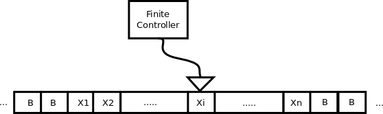
A Turing machine (TM) can be considered to be a FA-style “controller” coupled to a long tape instead of stack.
Finite automata recognized regular languages, a useful class of languages because they lead to many practical modeling applications and are closely related to the problem of lexical analysis in many programming languages.
Push-down automata recognized the context free languages, a useful class of languages because they correspond to the common syntactic structure of many programming langauges and structured input notations.
So what do we get by swapping out the stack of a PDA, on which we and read and write only at one end, with a tape on which we can move, read, & write at arbitrary locations? We actually get a machine that can carry out any algorithm.
- And that will, in turn, allow us to explore questions of just what kinds of problems can and cannot be solved using algorithms.
We say that a problem that cannot be solved by an algorithm is undecidable.
We will eventually see a set of well-known (and surprisingly practical) problems that can be proven to be undecidable.
We will then be able to prove new problems to be undecidable by the process of “reduction”.
Suppose that we have a problem $P_1$ that is known to be undecidable, and we have another problem $P_2$ that might or might not be undecidable.
If we can show that one way to solve $P_1$ would be to convert it (algorithmically) into an instance of problem $P_2$, so that if we could solve $P_2$ we would have solved $P_1$ as well. We call that conversion the reduction of $P_1$ to $P_2$. If we can find such a reduction, then if there is any algorithm that solves $P_2$, then there would also be an algorithm to solve $P_1$. Specifically that algorithm would be:
reduce P1 algorithmically to P2.
apply the P2-solving algorithm
So what we get is a kind of proof by contradiction. If we assume that an algorithm to solve $P_2$ exists and can show an algorithm that reduces any $P_1$ to a $P_2$ problem, then we could solve any $P_1$ problem. But that contradicts out initial statement that $P_1$ was known to be undecidable. Hence the assumption that an algorithm exists to solve $P_2$ must be false.
For example, we will eventually see that the problem:
For an arbitrary program P, is there an input that causes P to halt?
is undecidable. But suppose that we aren’t interested in that. Suppose that we are debugging a program, think that a particular line of code might be buggy, and just want to know if there is any input that actually reaches that line of code. Is there a program that we could run as a kind of debugger’s aid that would answer that question for us?
The answer is, “no”. Take an arbitrary program. Search though its code for any halt/exit statements. If the programming language says that a program can halt by reaching the end of its code, put a dummy statement there and add it to our list. Now, any program has a finite number of statements, so we will wind up with a finite number of statements in our list. We could go through them one by one and, if our “debugger’s aid” program existed, use it to see if any of our program halting statements can be reached by some input. We would then have solved the problem of whether the original program halted on some input. But that’s known to be undecidable, so our “debugger’s aid” program cannot exist.
2 The Basic Turing Machine
A Turing machine consists of a finite state controller, an infinitely long tape divided into cells, each cell capable of holding one symbol, and a read/write head that
- is positioned at some specific cell,
- can read the symbol at that cell and supply it to the controller as an input,
- can accept a symbol from the controller and write it into that cell, and
- can accept a signal from the controller to move one cell to the left or to the right of its current position.
A move of the Turing machine is a function of
- The current state of the finite controller
- The symbol under the read/write head.
In response to those inputs, the Turing machine may
- Change the controller state.
- Write a symbol onto the current cell of tape (replacing whatever is already there).
- Move the head one step to the left or to the right.
A move might leave the state unchanged. It might leave the tape unchanged (or, if you prefer, write the same symbol into the cell that is already there). It cannot, however, keep the read/write head stationary. it must move one cell either to the left or to the right.
2.1 The Formal Definition
A Turing machine is a 7-tuple
\[ M = \{ Q, \Sigma, \Gamma, \delta, q_0, B, F \} \]
where:
- $Q$ is the finite set of states of the controller,
- $\Sigma$ is a finite set of input symbols (symbols that ca be on the tape when we start).
- $\Gamma$ is the set of tape symbols, the input symbols plus possible additional symbols that can be written to the tape.
- $\delta$ is the transition function $\delta: Q \times \Gamma \Rightarrow Q \times \Gamma \times D$, where $D$ is a direction in $\{L,R\}$ (left or right).
- $q_0$ is the starting state for the controller.
- $B$ is a special symbol used to indicate “blank” spaces on the tape. Initially the tape must contain $B$ in all except a finite number of positions.
- $F$ is the subset of $Q$ denoting the final or accepting states of the controller.
The function $\delta$ expresses the transition that can be made given the current state and the current symbol under the tape head. For example, if
\[ \delta(q_1,x) = (q_2, y, R),\]
then when the controller is in state $q_1$ and the symbol under the tape head is ‘x’, the machine changes to state $q_2$, rewrites the ‘x’ with ‘y’, and then moves the head one step to the right.
You might take a certain comfort in the fact that the range of $\delta$ is $Q \times \Gamma \times D$ and not $\mathscr{P}(Q \times \Gamma \times D)$.
What does that tell you about the TM’s controller?
A common variant on this definition of TMs is to expand the set of Directions that the tape head can move from ${L, R}$ (left or right) to ${L, R, S}$ (left, right, or stationary). Many writers about TMs use this variation.
It really dosn’t change the power of the TM (the set of languages that it can recognize), because we can always simulate a “stationary” move by moving one step to the left or right, then moving back in the opposite direction without changing the symbol on the tape. E.g.,
we can replace this transition (If we are looking at a 0, rewrite it as a 1 and stay on the same cell)
with this two-transition sequence ((If we are looking at a 0, rewrite it as a 1 and move left, then move back to the right, leaving the cell on the left unchanged).
We’ll stick with the textbook’s convention of only using ${L, R}$ movements because some of the proofs use that as a simplifying assumption. But keep in mind that the “stationary” option is plausible and does not change the basic nature of the TM.
2.2 Accepting Strings
TMs “accept” differently than our earlier automata.
A TM can
- Halt, accepting, by reaching an accept/final state
- regardless of whether all input has been processed or not.
- Halt, failing, because no transition exists from the current state on the current input, or
- Run forever
2.3 Solving Problems with Turing Machines
We use a Turing machine by giving it an input string already written on the tape.
-
The tape head is initially positioned on the leftmost non-blank character of the input.
-
The Turing machine halts, accepting the input, if it ever enters a final or accepting state.
-
There is no requirement that the TM have read all of the input characters on the tape prior to halting.
-
-
The Turing machine halts, failing if it ever enters a non-accepting state from which no transition is defined for the current state and tape symbol.
In some instances, we think of TMs as computing functions rather than simply accepting/rejecting inputs. In such cases, we consider the contents of the tape when the TM halts (accepting) to be the result of the function.
2.4 Running a Turing machine
We can describe the current state of a TM by listing all of the non-blank characters to the left of the head, the current state, the symbol under the head, then all of the non-blank characters to the right of the head. For example, $xxyyyq_1xyy$ would describe a state which the controller is in state $q_1$, the tape has the the symbols ‘xxyyyxyy’, and the head is positioned over the rightmost ‘x’.
Question
If we are in state $xxyyyq_1xyy$ and if $\delta(q_1,x) = (q_2, y, R)$, then what state would we enter?
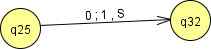
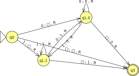
Here is a TM that is designed to work on a string of 0’s and 1’s, with the tape head positioned somewhere within the string. The table gives the move to be made for for each combination of state and symbol under the head:
| symbols | |||
|---|---|---|---|
| state | 0 | 1 | B |
| $q_0$ | ($q_1$,B,R) | ($q_2$,B,R) | ($q_3$,B,R) |
| $q_1$ | ($q_1$,0,R) | ($q_2$,0,R) | ($q_3$,0,R) |
| $q_2$ | ($q_1$,1,R) | ($q_2$,1,R) | ($q_3$,1,R) |
| $q_3$* | |||
but it’s probably easier to see what this does if we show a transition diagram instead.

For TMs, each transition is labeled with three components:
-
The first component is the (input) symbol under the tape head.
-
JFlap uses $\Box$ to denote blank symbols, which we tend to show as ‘B’ in text.
-
-
The second component is the replacement symbol to be written into the square before moving the head.
-
The third component is the direction (L or R) in which to shift the head.
Can you figure out what this TM does? Some hints:
- The state $q_1$ is entered whenever we have just seen a ‘0’.
- The state $q_2$ is entered whenever we have just seen a ‘1’.
- Whenever we leave state $q_1$, we always write a ‘0’.
- Whenever we leave state $q_2$, we always write a ‘2’.
Question Can you modify this TM so that, when it is done, it re-positions the head back at it’s starting position?
2.5 Programming Turing Machines
“Programming” a Turing machine is not an easy process. In my opinion, it calls for the same kind of skills that assembler language programmers use, and how many computer scientists do that on a regular basis anymore?
So in many cases you will see that your text uses arguments based upon shortcuts that are known to be valid programming styles for a TM.
2.5.1 Storage in the State
We can pretend that our finite controllers have some finite number of storage cells that can hold a symbol each.
We can do this by a “trick” that shows that it requires no change to the actual definition of a TM. Instead of labeling our states with simple names like $q_0, q_1, \ldots$, we label them with a tuple of a state identifier plus the symbols in the storage cells.
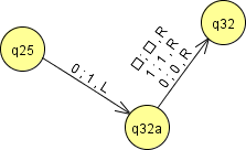
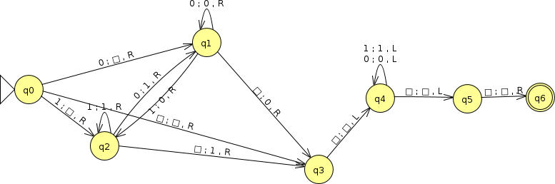
For example, I could modify our earlier shift-right TM by using a storage cell to remember the previously-read symbol:
| symbols | |||
|---|---|---|---|
| state | 0 | 1 | B |
| ($q_0$,x) | (($q_1,0)$,B,R) | (($q_1$,1),B,R) | ($(q_3,B)$,B,R) |
| ($q_1$,$x$) | (($q_1$,0),$x$,R) | (($q_1,1)$,x,R) | (($q_3,B)$,x,R) |
| $q_3$* | |||
This gives an illusion that we have lost a state, although, in fact, what we have done is really to replace…
… this machine by …
… by this one, which really only differs in the labels of the states.
Now, in this case, we’ve only “saved” one state by this trick. But, in general, a machine of $n$ states using $k$ cells, each of which can hold any of $m$ tape, could be equivalent to a “real” finite controller of up to $n k^m$ states.
2.5.2 Multiple Tracks
We can pretend that a TM has any finite number of tapes. Again, we can do this by a simple trick. In this case, we simulate $k$ tapes by replacing out tape alphabet $\Gamma$ by a list of all possible k-tuples of symbols from $\Gamma$. So, for example, if $\Gamma = \{0, 1, B\}$, we replace that by $\{(0,0), (0,1), (0,B), (1,0), (1,1), (1,B), (B,0), (B,1), (B,B) \}$.
- If you are uncomfortable with the notion that tuple can be a symbol, just imagine that we gave a separate symbol to each:
\[ \begin{eqnarray} \zeta & = & (0,0) \ \eta & = & (0,1) \ \theta & = & (0,B) \ \mu & = & (1,0) \ \nu & = & (1,1) \ \xi & = & (1,B) \ \rho & = & (B,0) \ \sigma & = & (B,1) \ \tau & = & (B,B) \ \end{eqnarray} \]
and use a new $\Gamma = \{\zeta, \eta, \theta, \mu, \nu, \xi, \rho, \sigma, \tau\}$.
Your text notes that a common programming style is to use one track for the main set of symbols being manipulated and another as a place to write markers to make it easy to shift back and forth to “remembered” positions.
2.5.3 Subroutines
Small specialized Turing machines can be embedded into a larger machine, much like subroutines in a programming language.
We could, for example, rewrite our earlier “shift right and then reposition” TM
as a combination of our original “shift right” TM and
this “shift left over all 0’s and 1’s” block, combining them like this:
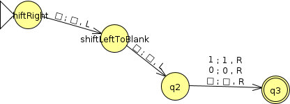
We “call” one of these subroutines by entering its initial state, but a TM has no mechanism for returning to its caller. So a better way to think of this might be as “building blocks”. If we wanted to use one of those blocks twice in one larger calculation, we would need to duplicate the entire set of states being reused.
3 Variations on Turing Machines
There are a couple of variations of Turing machines worth mentioning that your text shows are, in fact, equivalent to the basic Turing machine.
3.1 Multi-Tape TMs
We’ve already discussed multi-_track_ TMs, where the TM has multiple tapes, but the tape read/write heads in those are tied so that they all move left and right together.
A multi-tape TM, on the other hand, allows each tape head on multiple tapes to move independently.
Remember we talked about the possible third option of a TM allowing transitions that kept the head stationary? Although your text does not use that for ordinary one-track TMs, it does use it with multi-tape TMs.
That’s because, I suspect, programming a multi-tape TM can get ugly real fast if you ever find yourself with one tape head an odd number of spaces from where you want it to be while another is an even number of spaces from where you want it. If both heads have to move on every transition, there’s no way to move one an odd number of places while moving the other one an even number of places, no matter how you mix up the L’s and R’s. There’s ways to get around that (copying the contents of one tape one space to the left) but it’s a pain to deal with that sort of thing on a regular basis.
Your text shows that a multi-tape TM with $k$ tapes can be simulated via a multi-track TM with $2k$ tapes and $2k$ storage cells in its fintie controllers. The extra tapes are used to store a marker indicating the position of the the $k$ tape heads.
Each “move” of the multi-tape machine can be simulated by using a subroutine to move to the marker of each of the $k$ tapes, storing the symbol found there into the corresponding storage cell. Once all $k$ symbols have been loaded into the storage cells, we can carry out the transition of the multi-tape machine, storing the $k$ output values and the $k$ movement directions in the storage cells. Then it’s back to some useful subroutines, to visit the marker for each tape, write the output there, and move the marker as indicated in the storage cells.
It’s not fast, but it does simualte a multi-tape machine.
3.2 Nondeterministic TMs
Suppose we allow the finite controller to be non-deterministic. Now, we know that we can convert that to a DFA. But remember that much of the complication introduced by nondeterminism in PDAs was the need to track multiple possible input and stack states. Similarly, if the finite controller of a TM becomes non-deterministic, the resulting “simultaneous” states could be associated with different tape values.
Nonetheless, all non-deterministic TMs can be simulated by a deterministic TM.
4 Turing Machines vs Digital Computers
We’ve been dropping hints all along about the power of Turing machines.
If we ignore the fact that a real computer does not have infinite memory (and even that is questionable if you consider the possibility of swappable disk and tape drives), then it should be pretty clear that a TM simulator could be written in most common programming languages.
Less obvious, but still well accepted, is the idea that a TM can simulate a digital computer. I’ll point out a couple of things in support of this:
-
The fact that digital CPUs can do arithmetic and other word-oriented computations, while TMs can only read and write symbols, is not particularly significant. In fact, doing binary arithmetic is included among the examples and exercises in your text. So we could prepare a set of computer arithmetic subroutines and drop those into a TM whenever needed.
-
That leaves the structure of RAM as the major difference between digital computers and TMs. But, by now, you have read lots of descriptions of TMs shifting some number of positions to the left or right before moving on to another part of a calculation. It should not be hard to image a RAM-on-tape, a TM with a set of storage cells to hold an address, and subroutines to shift the tape head all the way to the left and then to count forward the number of symbols represented by that stored address. So finite address space can surely be simulated.
So a TM is, with just a bit of handwaving about finite storage, exactly as powerful as a digital computer.
In the next module we will explore the question of what problems can be solved via algorithms. That’s slightly different from the conclusion that we have just drawn, because we have not yet established that digital computers are themselves powerful enough to run all algorithms. But that’s what’s coming up.