

Turing Completeness
CS390, Spring 2024
Abstract
We have argued that Turing machines can compute precisely the class of problems that can be solved algorithmicly. We have argued that Turing machines can simulate simple computer architectures, and that computers can simulate Turing machines,
But, in a practical world, we don’t program Turing machines nor do most of us work at the machine code level on our computers.
In this final lesson, we explore the question of whether our programming languages actually embrace all of the computational power available to them, or whether a poor choice of language features can “cripple” a language.
We close with a case study in which the organization responsible for a language standard chose to deliberate modify the language to limit its computation power.
1 Turing Completeness
The Church-Turing thesis says that any real-world computation can be translated into an equivalent computation involving a Turing machine. This is something of an article of faith, but we’ve accumulated enough circumstantial evidence at this point to believe that Turing machines are equal in computation power to any digital computer (that has been provided with infinite secondary storage). Whether this thesis would hold up for more esoteric models of computation that might arise in, say, quantum computing, is a challenge for future generations of computer scientists.
Church’s original formulation of this thesis dates back to the 1930’s and stated that real-world calculation can be done using the $\lambda$-calculus, a mathematical formulation of pure functions based on recursion.
A programming language is said to be Turing complete or computationally universal if it can be used to simulate arbitrary Turing machines.
Most practical programming languages are Turing-complete. Writing a Turing machine simulator in most programming languages is a pretty straightforward task.
Then there are “computing environments” that you would not expect to be Turing Complete, but really are.
-
For example, Excel spreadsheets are Turing complete. That’s not entirely a surprise, since they include a full-fledged programming language for writing macros/extensions. But even without using that, the formula language of Excel can be argued to be Turing complete.1
-
The redstones in the game Minecraft define a language that is Turing-complete.
-
Conway’s Game of Life (with a demo here ), a much more amusing form of automaton than the ones we have focused on in this course, is also Turing complete.2
-
And, although it’s played for laughs, this presentation from CMU’s SIGBOVIK 2017, argues that PowerPoint is also Turing complete.
So what does a programming language need to have in order to be Turing complete?
We can set aside any idea that it relies on powerful arithmetic or logical computations embedded in the ALU. We’re seen that Turing machines have nothing like that – they rely simply on symbol matching and storage. Whatever we need, it’s mainly embedded in the control logic.
1.1 The Power of Iteration
The first high-level programming language, FORTRAN, featured control flow that was rather machine-code-like. It was basically a conditional jump. Any FORTRAN statement could be given a label, and the conditional statements in FORTRAN, roughly speaking amounted to
if (condition) go to statement-label
There was a “real” loop, a rather typical for-style loop using an integer counter, but that loop was limited to a finite number of repetitions. Since TMs can certainly go into an infinite loop, no programming language incapable of entering an infinite loop could possibly be Turing complete. However, these conditional jumps were more than adequate to develop a TM simulator.
Over time, though, people realized that this style of conditional jump might not be a very good way to write code, at least from the standpoint of readability and maintainability. The term “spaghetti code” was coined to describe programs whose various conditional and unconditional jumps were so complicated that any attempt to diagram them resulted in a tangled mess. There was a very real, practical interest in whether programming languages (and programmers) could accomplish the same computations with a simpler, more limited, set of control flow options.
The structured program theorem, also called the Boehm-Jacopini theorem, established3 that anything that could be computed using arbitrarily complicated control flows could also be computed using code that combined blocks of code in three specific ways:
- Executing one block of code and then another in sequence,
- Selection of one of two blocks of code based on the value of a boolean expression
- Executing a block of code until a boolean expression is true (iteration).
In practical terms, if a programming language permits straight-line sequences of code, some form of if-then-else, and some form of unbounded iteration (e.g., while loops), it is Turing complete.
1.2 The Power of Recursion
As noted earlier, FORTRAN was the first high-level programming language. The second is generally considered to be LISP.
LISP did not include unbounded iteration, but there was little doubt that it, too, was Turing-complete. Instead of iteration, LISP emphasized recursion. In fact, the declaration and execution of LISP functions was inspired directly by the $\lambda$-calculus, the same mathematical formulation used by Church in his original thesis. (In fact, the “keyword” in LISP that introduces a function is “lambda”.)
It’s a well-established fact that anything that can be done via iteration can be accomplished via recursion and vice-versa, and conversion between the two is something of a staple in data structures courses.
So we can reasonably expect that a programming language that features sequence, selection, and unbounded recursion will also be Turing complete.
2 A Case Study in Turing Completeness
Part I: The Postscript Programming Language
Not all programming languages are designed for full-fledged software development efforts. There are many “little languages” designed for
- special-purpose code
- fast development of “throw-away” programs
Postscript is a special-purpose language for preparing documents that mix text and graphics.
When laser printers capable of high-resolution graphics output came onto the market, coming up with a way to describe the desired output to the printer was a bit of a challenge. The “obvious” choice of generating a raster or bitmap of the desired image, transmitting that to the printer, and having the printer simply print that raster bit by bit, was unappealing:
-
It added a significant computational load to the computer that was driving the printer.
-
The resulting rasters were huge, and the time to simply transmit them from the computer to the printer would be prohibitively slow. If done over a network, this could result in a significant extra load on the network, slowing down the “main” operations of the computers on that network.
The solution was to send the printer, not a bitmap of the final image, but a program that could be executed on the printer’s own CPU to generate that bitmap. Postscript was the language designed for that purpose.
To understand why this approach might offer such a large improvement, consider the problem of printing a page full of text. On that page, a letter like ‘e’ in, say, a Times-Roman 11-pt font, might occur many dozens of times. If we were transmitting a complete bitmap. each of those occurrences of ‘e’ would add their own little 2D block of bits to the image. But, in Postscript, we would treat each letter in a font as a small function describing how to draw that letter. At worst, we might have to supply one copy of that 2D block of bits. A “font” could be nothing more than an array of such functions, indexed by the ASCII code of each character. A Postscript program to render that page of text would include repeated calls to the function in times-roman-font[101] (101 being the ASCII code for ‘e’). In fact, the program probably just supplies a array of ASCII codes for an entire line of text, looping through that array to pick up one character at a time and invoking the Times-Roman font “function” for each character in turn.
Not only does this permit a significant compression of the information to be transmitted to the printer, it also offloads the computation of the actual raster from the main computer onto the printer’s own CPU. It also provides a mechanism whereby fonts could be used whether pre-loaded into the printer or supplied with the as a data structure in the document’s program. Not at all coincidentally, Adobe, the inventor of Postscript, was in the business of designing and selling/licensing new fonts.
2.1 Postscript Overview
Postscript is a stack-based language. A Postscript program is, at its most basic, a list of operators and constants. As each of these is “executed”, it pulls some number of values from the top of a stack, then pushes its results or answers onto the top of that same stack.
For example, the Postscript code to evaluate the expression $10 (x+1)$ is
10 x 1 add mul
which executes like this:
  | 1 of 6 |   |
With so much emphasis on the stack, it’s not surprising that a number of the common operators are for manipulating or rearranging items on the stack:
Many of the most common operators in Postscript are for manipulating data on the stack:
| inputs | op | outputs | description |
|---|---|---|---|
| obj$_1$ | pop | Discard the top element from the stack. | |
| obj$_1$ obj$_2$ | exch | obj$_2$ obj$_1$ | Swap the top two elements on the stack. |
| obj$_1$ | dup | obj$_1$ obj$_1$ | Copy the top element on the stack. |
| obj$_n$ … obj$_0$ i | index | obj$_n$ … obj$_0$ obj$_i$ | Copies the $i^{\mbox{th}}$ element down on the stack, pushing the copy on top. |
| obj$_1$ … obj$_n$ n | copy | obj$_1$ … obj$_n$ obj$_1$…obj$_n$ | Copies the top $n$ elements on the stack. |
2.2 Data Types
Postscript data types start with numbers (integer and floating point). In addition to the add and mul operators already seen, there are
| inputs | op | outputs |
|---|---|---|
| num$_1$ num$_2$ | add | sum |
| num$_1$ num$_2$ | sub | difference |
| num$_1$ num$_2$ | mul | product |
| num$_1$ num$_2$ | div | quotient |
| int$_1$ int$_2$ | idiv | quotient |
| int$_1$ int$_2$ | mod | remainder |
| base exponent | exp | power |
| num$_1$ | abs | absolute-value |
| num$_1$ | neg | negation |
| num$_1$ | ceiling | num$_2$ |
| num$_1$ | floor | num$_2$ |
| num$_1$ | round | num$_2$ |
| num$_1$ | sqrt | num$_2$ |
| num$_1$ | atan | num$_2$ |
| num$_1$ | cos | num$_2$ |
| num$_1$ | sin | num$_2$ |
| num$_1$ | ln | num$_2$ |
| num$_1$ | log | num$_2$ |
Postscript supports strings, which are written inside parentheses (like this) instead of quotation marks.
It has arrays, which are created by using a special operator [ that pushes a “start of array mark”. This is followed by pushing an number of items onto the stack, then executing the end-of-array operator ‘]’, which collects all the items on that stack down to the ‘[’ into an array, leaving the reference to the array at the top of the stack.
Arrays can be joined to form matrices, which are key elements in many graphics calculations as ways to perform rotation and scaling.
“Procedures”, stored blocks of code, are created in a similar fashion but use { } instead of [ ].
Postscript has “dictionaries”, which are essentially hash tables that associate a string “name” with some arbitrary type of value.
- In addition to the operand stack, Postscript maintains a dictionary stack.
- When a name’s value is needed, the name is hunted in the top dictionary, then the next lower, then the next, until
- the name has been found
- or all dictionaries in the stack have been searched unsuccessfully
2.3 Assignment
Normally when we encounter a variable name like ‘x’, its value is pushed onto the stack. But Placing a ‘/’ in front of it causes the name itself, not its value, to be put on the stack.
This allows us to bind values to names.
Assignment is accomplished via the def operator. For example:
/x 42 def
assigned the value 42 to the variable x.
Functions are declared by assigning a procedure to a variable, e.g.,
/double { 2 * } def
2.4 Control Flow
Control flow in Postscript looks a bit strange at first, because of the stack-oriented model.
- We push the boolean condition expression
- Then we push the procedures we wish to choose among / iterate onto the stack
- Then we apply the appropriate control operator
2.4.1 Conditionals
The if operator introduces an if-then construct.
Example: x 0 lt { /x x neg def } if
The x 0 lt evaluates a condition (is $x < 0$?), leaving a boolean on the stack. The {...} is a procedure that becomes the then-part of the if. The if operator checks the boolean value and decides whether to execute the then-part procedure or to simply discard it.
Similarly, we have an ifelse operator that takes two procedures, one representing the then-part and the next representing the else=-part.
Example: x 0 lt { /absx x neg def} { /absx x def } ifelse
Question: How would you define your own absolute value function?
2.4.2 Loops
A simple bounded loop is provided by the repeats operator. For example,
16 { 2 mul } repeats
would execute the procedure inside the { } sixteen times.
Unbounded loops are provided by the loop operator, which repeats a procedure until the procedure invokes an `exit operator.
E.g.,
{ 1 sub   % subtract 1 from top item
  dup 0 le { exit } if % until it becomes 0
} loop
There is also a for-loop-like construction
| inputs | op | outputs | description |
|---|---|---|---|
| init incr limit proc | for | ||
start incr limit { ... } for
is equivalent to the C++ code:
for (tmp = init; tmp <= limit; tmp += incr)
{
  push tmp;
  proc;
}
Now, having established that Postscript has sequence, selection, and iteration, we could stop now and safely conclude that Postscript is Turing complete. Actually, it has recursion as well, so it’s doubly-qualified.
But, in case you’re wondering just why Postscript was useful for driving printers, let’s talk about the fun stuff.
2.5 Graphics
The basic concept of Postscript graphics is the path, a collection of virtual ink strokes on a page. Once you have created a path, there are several things that you can do with it.
-
You can draw (stroke) the path so that it appears on the printed page.
-
If the path is “closed” (starts and ends at the same point), you can fill the interior of the path with a color or pattern.
-
If the path is “closed”, you can use it as a “clipping” boundary for future drawing. It then functions as a kind of window so that any future drawing operations are only visible if they lie within the window.
Graphics in Postscript use a basic coordinate system that lower-left corner of the paper as $(0,0)$.
- The units are “points”, a traditional unit in typesetting, roughly $\frac{1}{72}$ of an inch.
- The current page is displayed (printed) and then cleared by the
showpageoperator.
For convenience, I will use the following function to convert from inches to points:
/inch { 72 mul } def
E.g, 1.5 inch puts $108$ on the stack.
2.5.1 Paths
The basic steps in drawing something are:
- Start a new path with
newpath - Create a path as a series of line segments and/or curves.
- Then do one or more of the following:
- draw the current path (
stroke) - fill the area enclosed by the path with a color (
fill) - clip all future images lying outside the path (
clip)
- draw the current path (
Drawing Lines
| inputs | op | outputs | description |
|---|---|---|---|
| x y | moveto | Sets the current position to $(x,y)$. Does not affect the path. | |
| x y | lineto | Adds to the current path a line segment from the current position to $(x,y)$. Then makes $(x,y)$ the current position. | |
| x y | rlineto | Adds to the current path a line segment from the current position $(x_c,y_c)$ to $(x_c+x, y_c+y)$. Then makes to $(x_c+x, y_c+y)$ the current position. | |
| closepath | Adds a line segment from the current position to the start of the path, marking the path as closed. |
A simple Postscript program to draw a box:

%!
%
% Draw a simple box.
%
/inch { 72 mul } def

newpath
0 0 moveto
0  1 inch lineto
1 inch  1 inch lineto
1 inch  0 lineto
0 0 lineto
stroke

showpage
Even with just lines, we can create some elaborate effects:
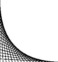
%!
newpath
0 200 % x, y
20
{
   exch
   dup 0 moveto
   exch
   dup 0 exch lineto
   stroke
   10 sub exch
   10 add exch
} repeat
showpage
Here is a function to draw a box at the current position:
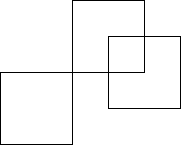
%!
/inch { 72 mul } def
/box {0 1 inch rlineto
      1 inch 0 rlineto
      0 -1 inch rlineto
      closepath } def

newpath
0 0 moveto box
1 inch 1 inch moveto box
1.5 inch 0.5 inch moveto box
stroke showpage
After the declaration of the function /box, we call it three times.
2.5.2 Color
Colors can be specified in RGB form, three values ranging from 0 to 1 each, for Red, Blue, and Green intensity.
| inputs | op | outputs | description |
|---|---|---|---|
| red green blue | setrgbcolor | Set current color, where each value ranges from $0$ to $1$. | |
| currentrgbcolor | red green blue | get the current color |
We can add a bit of color to our earlier examples:
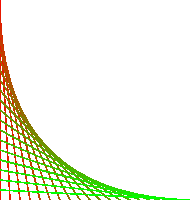
%!
newpath
0 200 % x, y
1 1 20
{  % red = 1-0.05i
   dup 0.05 mul 1 exch sub
   % green = 0.05i
   exch 0.05 mul
   % blue = 0
   0 setrgbcolor

   exch
   dup 0 moveto
   exch
   dup 0 exch lineto
   stroke
   10 sub exch
   10 add exch
} for
showpage
We can fill in a closed shape with the current color by using\
| inputs | op | outputs | description |
|---|---|---|---|
| fill |
instead of stroke.

%!
/box {dup 0 rlineto
      dup 0 exch rlineto
      neg 0 rlineto
      closepath } def
/irnd {rand exch mod} def
/rrnd {rand 1000 mod 1000 div} def
usertime srand
10 {
  newpath
  100 irnd 200 irnd moveto
  100 irnd  box
  rrnd rrnd rrnd setrgbcolor
  fill
} repeat
showpage

This actually uses a random number generator to select the box coordinates and colors, so it actually produces slightly different results each time it is executed.
2.5.3 Drawing Curves
| inputs | op | outputs | description |
|---|---|---|---|
| x y r ang$_1$ ang$_2$ | arc | Adds to the path a counterclockwise arc of a circle |
where $(x,y)$ is the center of the circle, $r$ is the radius, and the portion of the arc drawn is from angle $\mbox{ang}_1$ to $\mbox{ang}_2$ (measured in degrees).
%!
newpath
10 10 360
 {
  100 100         % x, y
  2 index 4 div   % r
  0               % ang1
  4 index         % ang2
  arc
  stroke
} for
showpage
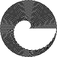
2.5.4 Clipping
One must often be careful not to go outside the bounds of a drawing area. One way to control this is to define a clipping path, beyond which graphics will not be drawn.
This is done with the operator clip.

%!
newpath
30 30 25 0 360 arc clip
newpath
0 200 % x, y
1 1 20
{
   dup 0.05 mul 1 exch sub
   exch 0.05 mul
   0 setrgbcolor

   exch
   dup 0 moveto
   exch
   dup 0 exch lineto
   stroke
   10 sub exch
   10 add exch
} for
showpage
In the first few lines, we create a circle as a path, then use the clip author to make that circle the limits for all subsequent graphics. The rest of the program is the same colored “fan” of lines that we demonstrated earlier.
2.6 What’s Interesting About Postscript
(Well, graphics are always flashy.)
-
It shows the power of a well-chosen set of special-purpose primitives
-
The language itself is simple and easily processed.
2.7 From Postscript to PDF
Postscript is powerful enough to compute some very complicated graphics, e.g., fractals. But, on the slow cheap CPUs embedded into many printers, such calculations could take a long time, giving an impression that the printer was no longer working.
Postscript is powerful enough to go into infinite loops, meaning that the printer truly is no longer working (until rebooted).
Now, most Postscript programs are not written by human programmers but are generated by printer drivers. But a buggy or poorly designed printer driver can certainly generate programs that hang forever or that take inordinately long times to prepare a page.
Printers are, in the minds of most users, simple appliances compared to “real” computers. The typical customer using a printer does not expect and will not understand that the printer is actually serving as a fully Turing-complete computing device and would likely blame the printer’s manufacturer for slow performance on Postscript from a poorly designed printer driver.
Adobe eventually created PDF as a successor to Postscript. Like Postscript, PDF is actually a programming language, so that printer drivers are sending programs, not raw images to printers.
We have to speculate a bit on what Adobe’s motivations were in designing PDF, but it seems clear to me that one of the things they were looking for was predictability – the running time of a program on a printer needed to be bounded and predictable. No infinite loops. No extraordinarily long computations.
At one level, PDF isn’t actually all that different from Postscript. It is still a stack-based programming language. Most of the PDF operators existed (under different names) in Postscript. In fact, the open-source Postscript processor ghostscript has long been able to can read and process PDF as well as the Postscript language it was originally designed to handle.
What are the major changes from Postscript to PDF?4
-
Many of the operators are given shorter names. Examples:
Postscript PDF stroke s moveto m lineto l close h fill f - Presumably, these shorter names reduce the overall program length and therefore the time required to transmit the program from the computer to the printer.
-
And, since these programs are not intended to be written or read by humans, the loss in readability is presumably not considered a problem.
-
- Presumably, these shorter names reduce the overall program length and therefore the time required to transmit the program from the computer to the printer.
-
The source code of a PDF program need not be entirely in plain text. After a short plain-text header, the bulk of the code can be compressed (binary) bytes, much as you would get by applying
zipor other archiving programs.-
Again, this is pretty clearly aimed at reducing the size of the programs that need to be transferred to the printer.
-
Truthfully, if they were going to do this, I’m not convinced there was much point in shortening all the command names. Most modern compression algorithms would have done as good or better a job of mapping repeatedly used command words onto single-byte values.
-
-
-
Procedures can no longer be bound to names and called as functions.
-
No programmer-named functions means no recursion.
-
-
The unbounded loop operator,
loop, was removed entirely.-
No unbounded loops means no infinite loops. The only iterations are fairly simple constructs that apply a procedure to each element of a finite array.
-
With no recursion and no unbounded loops, PDF is clearly not Turing complete. Adobe deliberately sacrificed computing power in favor of predictability. I don’t mean that as a criticism. It makes perfect sense in the context of “printer-as-appliance”. But it is, to my knowledge, the only time that a prominent programming language has been deliberately hobbled so that it would not be Turing complete.
Footnotes
1: Felienne Hermanns, Excel Turing Machine, http://www.felienne.com/archives/2974, Posted on September 19, 2013, retrieved on November 15, 2016
2: Paul Rendell, A Turing Machine in Conway’s Game of Life, http://rendell-attic.org/gol/tm.htm, January 12, 2005, retrieved 15 November 2016
3: Bohm, Corrado and Giuseppe Jacopini, Flow Diagrams, Turing Machines and Languages with Only Two Formation Rules, Communications of the ACM. 9 (5), May 1966, pp. 366–371, doi:10.1145/355592.365646.
4: Adobe Systems Incorporated, Document management – Portable document format – Part 1: PDF 1.7, 2008, available at http://wwwimages.adobe.com/content/dam/Adobe/en/devnet/pdf/pdfs/PDF32000_2008.pdf