


Undecidable Problems
CS390, Spring 2025
Abstract
If a Turing machine can solve any problem that can be solved by algorithms, then we can exploit TMs to explore the boundaries of what is and is not computable.
The class of undecidable problems represent the fundamental limits of what we can accomplish with digital computers.
1 Recursive and Recursively Enumerable Problems
We now come to what is, in many ways, the climax of the course. We are ready to directly address the fundamental question of what can be computed and what cannot.
We remain focused on decision problems, problems have a yes/no or true/false answer.
We will recognize three distinct classes of problems. These will be based upon two key definitions.
A problem is considered decidable or recursive if it can be solved by an algorithm, a Turing Machine that halts on all inputs after a finite amount of time.
-
This means that whether the answer to the problem is true or false, we will get an answer eventually.
-
The term “recursive” in this context has nothing to do with the idea of “recursive functions” in programming.
Problems that are not decidable are called undecidable.
However we will draw a distinction between two “levels” of undecidability, based upon the following idea:
A problem is recursively enumerable (RE) (a.k.a. semidecidable or partially decidable) if there exists a Turing machine that solves the problem in a finite time when the answer to the problem instance is “true” but might not halt in some case when the answer is “false”.
There are problems that are not even partially decidable, problems for which no Turing machine exists. There does not seem to be an accepted name for this class of problems. They are simply “undecidable problems that are not RE.”
1.1 Enumeration
The idea of “enumeration” is important enough to spend some time on it.
If we don’t have a way to decide, yes or no, whether a string is in a language, we can sometimes fall back on trying to find a procedure to list, or enumerate, the strings in that language.
However, before we get to such enumerative procedures, a simpler example of enumeration is worth noting:
We can enumerate all possible inputs to a Turing machine
The set of recursive/decidable problems is a subset of the set of RE/partially decidable problems. So our three levels of computability are:
-
decidable/recursive,
-
partially decidable/RE but not decidable/recursive, and
-
not partially decidable/RE.
2 Some Problems are not even Partially Decidable
We start by showing that there are problems for which no Turing machine exists that can even partially solve the problem in its “true” cases.
2.1 Encoding TMs
2.1.1 Non-limiting Assumption
Let’s make a few simplifying assumptions:
-
We will limit ourselves to problems with input alphabet 0,1. That’s not a big deal. As programmers, we are familiar with the the use of strings of bits to encode more complicated I/O structures, and know that this can be done without loss of generality.
-
We will still allow more than just those two symbols on the TM tape. In fact we need to, at the very least, allow blanks to appear on the tape.
-
-
We will also assume that our states are numbered q1,q2,…, with
-
q1 being the initial state.
-
q2 being the (only) final state.
It’s really not a limitation to have only one final state, because the TM is considered to halt immediately upon entering a final state. Given that, we really don’t need more than one.
-
-
We will assume that our tape symbols X1,X2,…, are arranged so that
- ‘0’ is X1
- ‘1’ is X2
- ‘B’ is X3
The other symbols may appear in any order after these.
Hopefully, you will agree that none of these assumptions limit the computing power of our TMs in any fashion.
Now, if you compare what we have done so far against our formal definition of a TM, you can see that we are now dealing with a TM of the form
M={Q,{0,1},{X1,X2,X3,…},δ,q1,X3,q2}
2.1.2 Encoding a TM as Tuples of Integers
We are almost at a point where we could do away with all of the letters in our TM description and just specify everything using positive integers. We’ve imposed a standardized numbering on the states and the input and tape symbols. We haven’t touched the transition function δ yet, though.
Remember that this function has the signature:
δ:Q×Γ⇒Q×Γ×D
We’ve already numbered all of the elements of Q and Γ. D has only two elements, the directions L and R. Let’s agree to order them as D1=L,D2=R. So any transition in δ can now be expressed as a tuple of 5 integers. For example, if δ(q1,0)=(q4,B,L), we could encode that transition as (1,1,4,3,1). The first two 1’s designate the inputs q1 and X1=0, and the final three numbers denote q4, X3=B, and D1=L.
That means that the entire δ function can be encoded as a set of 5-tuples of integers.
2.1.3 Encoding a TM on a Tape
So everything is now down to positive integers now. For this we just need to establish a few conventions.
We can next consider the problem of writing an entire TM onto a TM tape using only 0’s and 1’s. Now, again, programmers should have few problems believing that numbers can be readily converted to binary forms. You may even be aware already that there are more than one way to do so. The complicating factors here are that, although we know that the number of states and the number of tape symbols for any given TM will be finite, there is no upper limit to we can’t predict, in advance, how many bits per number we will need. Similarly, we know that the number of transitions (now, 5-tuples) in δ would be bounded above by |Q|×|X|, but we don’t know, in advance, how large that number will be.
So we won’t use the “conventional” binary format for our numbers. Instead we will use a unary format in which the number n is represented as a string of n zeros. We will use the ‘1’ character as a “fencepost” to delimit the start and end of a number, also serving to separate adjacent numbers.
For example, earlier we said that the transition δ(q1,0)=(q4,B,L) could be encoded as (1,1,4,3,1). On a TM tape, we would write this as
1010100001000101
Count the zeros.
Now, obviously, this is a terrible encoding from a standpoint of readability by humans. But that’s no more relevant here than would the argument be that binary machine code is nearly unreadable by humans. We don’t do these encodings to document the behavior for humans; we do them to make those behaviors something that can be automatically processed.
To write the entire δ function to a tape, we will adopt a convention of starting/ending/separating each 5-tuple denoting a single transition by 11, so that inter-transition boundaries are more easily distinguished from inter-integer boundaries.
For example, if our TM has transitions δ(q1,0)=(q4,B,L), encoded as (1,1,4,3,1), and δ(q1,1)=(q3,1,L), encoded as (1,1,3,2,1), we might find the following inside our δ function when it is written to a tape:
110101000010001011010010001001011
Now, if we write the δ function to a tape, we really don’t need to write anything else. Referring to our definition of a TM again:
M={Q,Σ,Γ,δ,q0,B,F}
we can infer the number of states (QQ) and tape symbols (Γ) from the entries in δ, and our non-limiting assumptions have standardized the values for Q0, B, and F.
Having mapped a Turing machine onto binary integers leads to an interesting conclusion:
We can enumerate the set of all possible Turing machines
2.2 Diagonalization
Diagonalization is an interesting proof technique that pops up in a lot of problems involving infinite sets.
For example, Cantor used it in 1891 to prove that the set of real numbers is not countable (i.e., that although both the set of integers and the set of real number are infinite, there is a sense in which there are “more” real numbers than integers). Some people think that’s intuitively obvious. Others, particularly those who have seen Hilbert’s paradox of the infinite hotel, are surprised that this is true.
The argument goes like this. Suppose that the real numbers are countable – that we can put them into a one-to-one correspondence with the set of integers. In that case, we could write out an infinite list of just the decimal parts of those numbers, in order by their integer equivalents. We will extend each number out to an infinite number of decimal places, padding with zeroes if necessary. So we might get something like this:
1 .0000000000000...
2 .1000000000000...
3 .3333333333333...
4 .1415926535897...
5 .1231231231231...
⋮  ⋮
We can then prove that there is at least one positive real number, that is not in the list and not associated with any integer. We form that number by plucking the digits from the “diagonal” of the table (.00352…) and adding 1 to each digit, modulo 10 (.11463…).
The resulting number cannot possibly be in our list because, if you were to claim that it is in line j of the table, it would by definition have a different value in the jth digit. Hence there will always be some real numbers left uncounted in any attempt to associate them one-to-one with the integers.
We’re going to use a similar argument to show that a problem exists that cannot be even partially decided by any Turing machine.
2.3 The language Ld
Let Ld be the set of all binary encodings of TMs that do not accept (i.e., that fail or never halt on) their own encoding when presented it as an input.
OK, it’s a bit odd. But still, a binary encoding is just a string, and any set of strings is a language.
Is there a TM that accepts Ld?
- This question gives us two “levels” of TM. There are the TMs that are in the encodings and now another that decides wither they belong in this set of strings.
-
If the idea of a TM that decides problems about other TMs seems strange, ask yourself what programs like compilers or debuggers are, if not programs that operate on other programs?
-
Now, let’s make a table. On each axis of the table we will list all TMs, encoded as described above, in some order. The very existence of our encoding means that the set of all TMs is countable, because we have mapped them onto binary integers.
In the (i,j) entry of the table, we put a 0 if TMj accepts the binary encoding of TMi as input.
Question: Is there a TM somewhere in that list that accepts Ld?
Answer: No, there can’t be.
Consider the diagonal elements of that table. Those (i,i) elements describe the TMs that accept themselves (i.e., their own numeric encoding) as input.
Now form a string D as the complement of the diagonal elements. The elements of this string with 1’s would then be the strings/TMs in Ld.
Is there a TM, somewhere in this table, that computes D? Suppose we believed that TMk computed D. The row k of the table would be D. But we know that we formed Dk by taking the complement of element (k,k), so they can’t possibly be equal. Hence there cannot be any TM in the table that has D as its row.
Therefore there cannot be a TM that computes D. Therefore there is no TM that accepts Ld.
This is an example of a problem that is not even partially decidable.
3 Some Undecidable Problems are Partially Decidable
Next we will show that there is an intermediate level between decidable and no-turing-machine exists - the partially solvable or RE problems that are not decidable.
Now, any programmer is familiar with code that doesn’t always terminate. Who hasn’t written an infinite loop by mistake?
But we need to distinguish between problems that are partially solvable versus programs that might not halt.
Consider, for example, the problem of deciding whether a regular language L is non-empty. One approach to doing this, given a DFA for the language, would be something along the lines
// generate all possible input strings in Sigma*
//   in lexicographic order
w = "";
while (true) {
    if (DFA.accepts(w)) {
        return true;
    }
    w = next string in Sigma*;
}
Now clearly if the language is non-empty, this will eventually return true. Just as clearly, it does not halt when the language is empty.
This is not an algorithm by our definition. it certainly looks like it matches our concept of a recursively enumerable (partially decidable).
But, actually, this is just poor programming. Just because this code fails to halt on empty languages does not mean that all codes to solve this problem must do so. In fact, we have previously given a true algorithm for this problem that always halts in O(n) time where n is the number of transitions in the DFA. So the problem of determining whether a regular language is empty or non-empty is decidable even if some bad solution attempts might not live up to that requirement.
It’s trickier to show that a problem can only be solved by TMs that are, at best, guaranteed to halt on “true” outputs.
3.1 The Universal Turing Machine
We’ve already talked about the idea of writing a TM simulator program in a conventional programming language. And we’ve talked about the ability of TMs to simulate digital computers. And, in practical terms, we’re living in a time when virtual machines are no longer rare oddities but are used on a regular basis.
So all in all, it should not come as a big surprise that we can write a TM simulator, not just in a modern programming language, but in Turing machines.
Suppose we take a TM tape and write onto it a binary encoding of a TM and then, separated by a fence of 3 1’s, a binary input string. So the total input has the form M111w with M the encoded TM and w the input string. This would serve as the input to a Universal Turing machine (UTM), a TM simulator that accepts the string if the encoded machine M would have.
Your text gives the details of the construction of a UTM using a multi-tape TM. I won’t comment further on that because there’s little surprising about it. It’s just a grind to get it all “programmed” into a TM.
Consider the language consisting of all M111w inputs that describe a machine M that would accept the string w. Call this language Lu.
The UTM that is constructed in the text is one specific implementation of a TM to solve this problem. It is an implementation that accepts strings in finite time when M would, that fails in finite time when M would, and that does not halt on those inputs where M would not.
The question is, is this just bad programming or is it inherent in the problem itself that a “smarter” implementation cannot exist that would figure out, in finite time, whether or not M would eventually halt?
3.2 Lu is Not Recursive
Assume, for the sake on contradiction, that we have a TM M that decides the problem of whether a string is in Lu.
Now, let’s return to an earlier problem. Given an input w, can we decide if w∈Ld? The following would work:
-
See if w is a syntactically valid encoding of a TM (0’s and 1’s arranged with the appropriate 1 and 11 fence posts). If not, it’s not a TM that accepts anything, so it is in Ld. return true.
-
If w is syntactically valid, feed the string w111w to our machine M.
Because we are surmising that M is recursive$, we get a true/false answer in finite time. Return the complement of that answer.
This is clearly a recursive algorithm if M is. But we have already established that Ld is not recursive. So the assumption that a recursive M exists must be false.
So the problem of determining membership in Lu cannot possibly be recursive.
On the other hand, the construction of a UTM proves that Lu is, at the very least, recursively enumerable.
So this problem falls into that intermediate state - it is RE but not recursive.
4 Three TM Outcomes – Three classes of languages
When a TM is run on an input, three things can happen
- It may halt and accept the input.
- It may halt and reject the input.
- It may run forever.
This leads to three interesting classes of languages:
-
The recursive languages (RL) are ones for which there is a TM that accepts the language, always halting with an accept/reject answer.
- These are also known as decidable languages.
- We reserve the term algorithm for this class of problems.
-
The recursively enumerable languages (RE) are ones for which there is a TM that always halts accepting strings in the language, but for strings not in the language might halt rejecting the string or might run forever.
-
The semidecidable languages are the ones that are RE but not R.
-
-
Non-RE languages are languages for which there is no TM that accepts the language even in the limited, RE sense.
All regular and CFL are decidable.
4.1 Proof by Reduction
One of the most powerful tools we have for showing that a language is not recursive (or recursively enumerable) is reduction.
If we want to prove that a problem P is not recursive, we can do it by:
- Find another problem,
Q, that is already known to be not recursive. - Give an algorithm that, in finite time, converts any problem of type
Qinto a problem of typeP.This is called “reducing Q to P”.
-
Now we do a proof-by-contradiction. Assume, by way of contradiction, that
Preally is recursive. There must, by definition, be some Turing machineMthat accepts or rejects inputs toPin finite time.Then any time we wanted to solve a problem of type
Q, we could apply our reduction algorithm to convert it, in finite time, into a problem of typeP, then apply the Turing machineMso solve thatPproblem in finite time.The net result is that we now have a procedure for solving all problems of type
Qin finite time. But we choseQspecifically because we knew that no such procedure could possibly exist. This is a contradiction, and we are forced to conclude that our assumption thatPis recursive was incorrect.
With minor changes, we can apply the same reduction technique to proofs that certain problems are not recursively enumerable.
5 Rice’s Theorem
At this point you might be thinking that we have a long slog ahead of us to determine, one at a time, whether various properties of TMs are recursive, recursive enumerable, or neither.
Rice’s theorem will give us a shortcut.
Suppose we were interested in certain “properties” of languages. What would we mean by that? If I talk about blue-eyed people, or months with 31 days, or songs by my favorite band, I’m really giving you a shorthand name for a (sub)set of those things.
So a property of languages is just a set of languages. Examples would include, of course, the property of being Regular, or Context-Free, or recursive.
We will say that a property of the RE languages is trivial if it is always true (i.e., all RE languages are included) or always false (i.e., no RE languages are included).
Rice’s Theorem: Every non-trivial property of the RE languages is undecidable.
Let’s be clear about what this does and does not say.
This does not mean that all non-trivial questions about specific languages are undecidable. For example, consider the language {0,1,00}. We can certainly decide whether a given string w is in the language or not. in fact, it’s hard to imagine there’s much about this language that couldn’t be decided.
But that’s a language, not a set of languages, so it isn’t a property and isn’t covered by Rice’s theorem.
OK, consider the set of languages consisting only of that language: {{0,1,00}}. Now we have a property, and it’s non-trivial. Does Rice’s theorem really apply here? Did the extra set of {} really make this so much more mysterious?
Yes, because Rice’s theorem deals with properties of RE languages, and we specify an RE language by giving a TM for it, we are now obligated to determine whether or not a given TM accepts the language {0,1,00}. And that’s hard enough to be an RE problem of its own.
-
Again, let’s be careful. I am not saying that it’s hard to construct a TM to accept that language.
-
But if I walk up to you with a messy, complicated TM, and assert that it accepts that language, you might have a hard time determining whether my claim was correct. If I present you with ever more complicated TMs, you might not be able to prove or disprove my claim about the nastier ones. And that’s not a slam at your mathematical skills. No TM can do that either.
Another text1 states Rice’s Theorem in a slightly different form that I think may be helpful:
Rice’s Theorem: Let P be any nontrivial property of the language of a Turing machine. In other words, let P be a language consisting of Turing machine descriptions. P is undecidable if P fulfills two conditions:
- P is nontrivial – it contains some, but not all, TM descriptions.
- P is a property of the TM’s language — whenever L(M1)=L(M2), then M1∈P iff M2∈P.
Remembering that the RE languages are precisely those that can be recognized by TMs (that do not, necessarily, halt) and that we achieve the apparently difficult task of enumerating those languages by enumerating the possible encodings of TMs, it’s a little clearer in this formulation just what we mean by a property of the RE languages. The explicit statement of the second condition also helps to exhibit the difference between a property of the language versus a property of the TM.
For example, you can give me a Turing machine M that accepts the language L={0,1,00} and if you have kept that TM simple, I might be able to prove that it accepts exactly those three strings and no others. But Rice’s theorem doesn’t come into play on the proof of a property of a single TM. Rice’s theorem tells us I cannot list all Turing machines whose language is equal to L(M), i.e., that the property "accepts L={0,1,00} is not decidable.
5.1 Proof
The proof is in the text. I really want to comment mainly on a couple of the insights arrived at along the way to the proof:
The set of recursive problems is closed under complement.
If I can get a a decision, in finite time, on whether or not w is in L, then i can also get a decision on whether w is not in LL.
The set of recursively enumerable problems is not closed under complement.
These are problems for which the best possible TMs are not guaranteed to halt when w∉L. So it makes sense that we cannot guarantee that any TM would halt when w∈ˉL.
If a language L and its complement ˉL are both recursively enumerable, then they are recursive.
Suppose that M1 is guaranteed to accept strings in L in finite time and that M2 is guaranteed to accept strings in ˉL in finite time. We could simply run them in parallel on the same input string, knowing that one of them must accept in finite time and then shut down the other. Thus we will learn, in finite time, whether or not w is in L or not.
5.2 Applications of Rice’s Theorem
From Rice’s theorem, we can conclude that a whole host of TM-related problems are undecidable, including:
- Is L(M) a regular language?
- Is L(M) a CFL?
- Is L(M) empty?
- Does L(M) include any palindromes?
6 Implications for Software Developers
 "
"
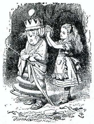
“I’m just one hundred and one, five months and a day.”
“I can’t believe that!” said Alice.
“Can’t you?” the Queen said in a pitying tone. “Try again: draw a long breath, and shut your eyes.”
Alice laughed. “There’s no use trying,” she said: “one can’t believe impossible things.”
“I daresay you haven’t had much practice,” said the Queen. “When I was your age, I always did it for half-an-hour a day. Why, sometimes I’ve believed as many as six impossible things before breakfast.”.
– Lewis Carroll, Alice through the Looking Glass
The kinds of reduction we used in proving that Lu was not recursive can be applied to many practical problems that software developers face on a regular basis.
-
Will this program always halt? (i.e., is it solving a decidable problem?)
-
I’m about to run a test. Will it halt on this input?
-
Is this block of code “dead”? In other words, is it true that no matter what input we present to this program, execution will reach this particular statement?
-
Do these two programs compute the same function?
-
Is this program correct (i.e., does this program compute the same function as its specification)?
In fact, almost all execution-behavior-related properties we can think of are likely to be undecidable for programs in general.
Yet, these aren’t obscure questions. These are problems that we face on a regular basis whenever we develop, test, and maintain software.
A good software engineer, I maintain, must often solve six undecidable problems before lunch-time.
We may be able to answer them for specific programs. We may be able to use our “true” (as opposed to “artificial”) intelligence or human intuition to leap to convincing answers in most cases.
But we cannot ever hope to devise “smart compilers” or other automatic aids that would answer these questions for programs in general. That’s the practical lesson of undecidability.
1: Sipser, Introduction to the Theory of Computation, 3rd ed., 2013, Cengage